5.40: The Zeta Distribution

\(\newcommand{\P}{\mathbb{P}}\) \(\newcommand{\E}{\mathbb{E}}\) \(\newcommand{\var}{\text{var}}\) \(\newcommand{\skw}{\text{skew}}\) \(\newcommand{\kur}{\text{kurt}}\) \(\newcommand{\N}{\mathbb{N}}\) \(\newcommand{\R}{\mathbb{R}}\) \( \newcommand{\Li}{\text{Li}} \)

The zeta distribution is used to model the size or ranks of certain types of objects randomly chosen from certain types of populations. Typical examples include the frequency of occurrence of a word randomly chosen from a text, or the population rank of a city randomly chosen from a country. The zeta distribution is also known as the Zipf distribution, in honor of the American linguist George Zipf.

Basic Theory

The Zeta Function

The Riemann zeta function \(\zeta\), named after Bernhard Riemann, is defined as follows: \[ \zeta(a) = \sum_{n=1}^\infty \frac{1}{n^a}, \quad a \in (1, \infty) \]

You might recall from calculus that the series in the zeta function converges for \(a \gt 1\) and diverges for \(a \le 1\).

Figure \(\PageIndex{1}\): Graph of \( \zeta \) on the interval \( (1, 10] \)

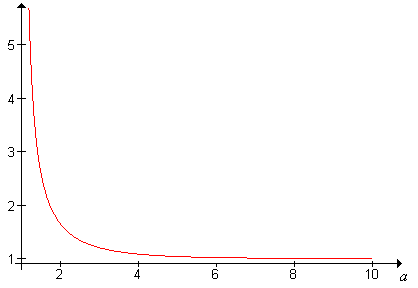
The zeta function satifies the following properties:

1. \(\zeta\) is decreasing.
2. \(\zeta\) is concave upward.
3. \(\zeta(a) \downarrow 1\) as \(a \uparrow \infty\)
4. \(\zeta(a) \uparrow \infty\) as \(a \downarrow 1\)

The zeta function is transcendental, and most of its values must be approximated. However, \(\zeta(a)\) can be given explicitly for even integer values of \(a\); in particular, \(\zeta(2) = \frac{\pi^2}{6}\) and \(\zeta(4) = \frac{\pi^4}{90}\).

The Probability Density Function

The zeta distribution with shape parameter \( a \in (1, \infty) \) is a discrete distribution on \( \N_+ \) with probability density function \( f \) given by. \[ f(n) = \frac{1}{\zeta(a) n^a}, \quad n \in \N_+ \]

1. \( f \) is decreasing with mode \( n = 1 \).
2. When smoothed, \( f \) is concave upward.

Proof

Clearly \( f \) is a valid PDF, since by definition, \( \zeta(a) \) is the normalizing constant for the function \( n \mapsto \frac{1}{n^a} \) on \( \N_+ \). Part (a) is clear. For part (b), note that the function \( x \mapsto x^{-a} \) on \( [1, \infty) \) has a positive second derivative.

Open the special distribution simulator and select the zeta distribution. Vary the shape parameter and note the shape of the probability density function. For selected values of the parameter, run the simulation 1000 times and compare the empirical density function to the probability density function.

The distribution function and quantile function do not have simple closed forms, except in terms of other special functions.

Open the special distribution calculator and select the zeta distribution. Vary the parameter and note the shape of the distribution and probability density functions. For selected values of the parameter, compute the median and the first and third quartiles.

Moments

Suppose that \( N \) has the zeta distribution with shape parameter \( a \in (1, \infty) \). The moments of \( X \) can be expressed easily in terms of the zeta function.

If \( k \ge a - 1 \), \( \E(X) = \infty \). If \( k \lt a - 1 \), \[\E\left(N^k\right) = \frac{\zeta(a - k)}{\zeta(a)}\]

Proof

Note that \[ \E\left(N^k\right) = \sum_{n=1}^\infty n^k \frac{1}{\zeta(a) n^a} = \frac{1}{\zeta(a)} \sum_{n=1}^\infty \frac{1}{n^{a - k}}\] If \( a - k \le 1 \), the last sum diverges to \( \infty \). If \( a - k \gt 1 \), the sum converges to \( \zeta(a - k) \)

The mean and variance of \(N\) are as follows:

1. If \( a \gt 2 \), \[\E(N) = \frac{\zeta(a - 1)}{\zeta(a)}\]
2. If \( a \gt 3 \), \[\var(N) = \frac{\zeta(a - 2)}{\zeta(a)} - \left(\frac{\zeta(a - 1)}{\zeta(a)}\right)^2\]

Open the special distribution simulator and select the zeta distribution. Vary the parameter and note the shape and location of the mean \( \pm \) standard deviation bar. For selected values of the parameter, run the simulation 1000 times and compare the empirical mean and standard deviation to the distribution mean and standard deviation.

The skewness and kurtosis of \(N\) are as follows:

1. If \( a \gt 4 \), \[ \skw(N) = \frac{\zeta(a - 3) \zeta^2(a) - 3 \zeta(a - 1) \zeta(a - 2) \zeta(a) + 2 \zeta^3(a - 1)}{[\zeta(a - 2) \zeta(a) - \zeta^2(a - 1)]^{3/2}} \]
2. If \( a \gt 5 \), \[ \kur(N) = \frac{\zeta(a - 4) \zeta^3(a) - 4 \zeta(a - 1) \zeta(a - 3) \zeta^2(a) + 6 \zeta^2(a - 1) \zeta(a - 2) \zeta(a) - 3 \zeta^4(a - 1)}{\left[\zeta(a - 2) \zeta(a) - \zeta^2(a - 1)\right]^2} \]

Proof

These results follow from the general moment result above and standard computational formulas for skewness and kurtosis.

The probability generating function of \( N \) can be expressed in terms of the polylogarithm function \( \Li \) that was introduced in the section on the exponential-logarithmic distribution. Recall that the polylogarithm of order \( s \in \R \) is defined by \[ \Li_s(x) = \sum_{k=1}^\infty \frac{x^k}{k^s}, \quad x \in (-1, 1) \]

\( N \) has probability generating function \( P \) given by \[ P(t) = \E\left(t^N\right) = \frac{\Li_a(t)}{\zeta(a)}, \quad t \in (-1, 1) \]

Proof

Note that \[ \E\left(t^N\right) = \sum_{n=1}^\infty t^n \frac{1}{n^a \zeta(a)} = \frac{1}{\zeta(a)} \sum_{n=1}^\infty \frac{t^n}{n^a} \] The last sum is \( \Li_a(t) \).

Related Distributions

In an algebraic sense, the zeta distribution is a discrete version of the Pareto distribution. Recall that if \( a \gt 1 \), the Pareto distribution with shape parameter \( a - 1 \) is a continuous distribution on \( [1, \infty) \) with probability density function \[ f(x) = \frac{a - 1}{x^a}, \quad x \in [1, \infty) \]

Naturally, the limits of the zeta distribution with respect to the shape parameter \( a \) are of interest.

The zeta distribution with shape parameter \( a \in (1, \infty) \) converges to point mass at 1 as \( a \to \infty \).

Proof

For the PDF \( f \) above, note that \( f(1) = \zeta(a) \to 1 \) as \( a \to \infty \) and for \( n \in \{2, 3, \ldots\} \), \( f(n) = 1 \big/ n^a \zeta(a) \to 0 \) as \( a \to \infty \)

Finally, the zeta distribution is a member of the family of general exponential distributions.

Suppose that \(N\) has the zeta distribution with parameter \(a\). Then the distribution is a one-parameter exponential family with natural parameter \(a\) and natural statistic \(-\ln N\).

Proof

This follows from the definition of the general exponential distribution, since the zeta PDF can be written in the form \[ f(n) = \frac{1}{\zeta(a)} \exp(-a \ln n), \quad n \in \N_+ \]

Computational Exercises

Let \(N\) denote the frequency of occurrence of a word chosen at random from a certain text, and suppose that \(X\) has the zeta distribution with parameter \(a = 2\). Find \(\P(N \gt 4)\).

Answer

\(\P(N \gt 4) = 1 - \frac{49}{6 \pi^2} \approx 0.1725\)

Suppose that \(N\) has the zeta distribution with parameter \(a = 6\). Approximate each of the following:

1. \(\E(N)\)
2. \(\var(N)\)
3. \( \skw(N) \)
4. \( \kur(N) \)

Answer

1. \(\E(N) \approx 1.109\)
2. \(\var(N) \approx 0.025\)
3. \( \skw(N) \approx 11.700 \)
4. \( \kur(N) \approx 309.19 \)