3.3: Mixed Distributions
- Page ID
- 10143
In the previous two sections, we studied discrete probability meausres and continuous probability measures. In this section, we will study probability measure that that are combinations of the two types. Once again, if you are a new student of probability you may want to skip the technical details.
Basic Theory
Definitions and Basic Properties
Our starting point is a random experiment modeled by a probability space \((S, \mathscr S, \P)\). So to review, \(S\) is the set of outcomes, \(\mathscr S\) the collection of events, and \(\P\) the probability measure on the sample space \((S, \mathscr S)\). We use the terms probability measure and probability distribution synonymously in this text. Also, since we use a general definition of random variable, every probability measure can be thought of as the probability distribution of a random variable, so we can always take this point of view if we like. Indeed, most probability measures naturally have random variables associated with them. Here is the main definition:
The probability measure \(\P\) is of mixed type if \(S\) can be partitioned into events \(D\) and \(C\) with the following properties:
- \(D\) is countable, \(0 \lt \P(D) \lt 1\) and \(\P(\{x\}) \gt 0\) for every \(x \in D\).
- \( C \subseteq \R^n \) for some \( n \in \N_+ \) and \(\P(\{x\}) = 0\) for every \(x \in C\).
Details
Recall that the term partition means that \(D\) and \(C\) are disjoint and \(S = D \cup C\). As alwasy, the collection of events \(\mathscr S\) is required to be a \(\sigma\)-algebra. The set \( C \) is a measurable subset of \( \R^n \) and then the elements of \( \mathscr S \) have the form \( A \cup B \) where \( A \subseteq D \) and \( B \) is a measurable subset of \( C \). Typically in applications, \( C \) is defined by a finite number of inequalities involving elementary functions.
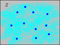
Often the discrete set \(D\) is a subset of \(\R^n\) also, but that's not a requirement. Note that since \(D\) and \(C\) are complements, \(0 \lt \P(C) \lt 1\) also. Thus, part of the distribution is concentrated at points in a discrete set \(D\); the rest of the distribution is continuously spread over \(C\). In the picture below, the light blue shading is intended to represent a continuous distribution of probability while the darker blue dots are intended to represents points of positive probability.

The following result is essentially equivalent to the definition.
Suppose that \(\P\) is a probability measure on \(S\) of mixed type as in (1).
- The conditional probability measure \(A \mapsto \P(A \mid D) = \P(A) / P(D)\) for \(A \subseteq D\) is a discrete distribution on \(D\)
- The conditional probability measure \(A \mapsto \P(A \mid C) = \P(A) / \P(C)\) for \(A \subseteq C\) is a continuous distribution on \(C\).
Proof
In general, conditional probability measures really are probability measures, so the results are obvious since \(\P(\{x\} \mid D) \gt 0\) for \(x\) in the countable set \(D\), and \(\P(\{x\} \mid C) = 0\) for \(x \in C\). From another point of view, \(\P\) restricted to subsets of \(D\) and \(\P\) restricted to subsets of \(C\) are both finite measures and so can be normalized to producte probability measures.
Note that \[\P(A) = \P(D) \P(A \mid D) + \P(C) \P(A \mid C), \quad A \in \mathscr S\] Thus, the probability measure \(P\) really is a mixture of a discrete distribution and a continuous distribution. Mixtures are studied in more generality in the section on conditional distributions. We can define a function on \(D\) that is a partial probability density function for the discrete part of the distribution.
Suppose that \(\P\) is a probability measure on \(S\) of mixed type as in (1). Let \(g\) be the function defined by \(g(x) = \P(\{x\})\) for \(x \in D\). Then
- \(g(x) \ge 0\) for \(x \in D\)
- \(\sum_{x \in D} g(x) = \P(D)\)
- \(\P(A) = \sum_{x \in A} g(x)\) for \(A \subseteq D\)
Proof
These results follow from the axioms of probability.
- \(g(x) = \P(\{x\}) \ge 0\) since probabilities are nonnegative.
- \(\sum_{x \in D} g(x) = \sum_{x \in D} \P(\{x\}) = \P(D)\) by countable additivity.
- \(\sum_{x \in A} g(x) = \sum_{x \in A} \P(\{x\}) = \P(A)\) for \(A \subseteq D\), again by countable additivity.
Technically, \(g\) is a density function with respect to counting measure \(\#\) on \(D\), the standard measure used for discrete spaces.
Clearly, the normalized function \(x \mapsto g(x) / \P(D)\) is the probability density function of the conditional distribution given \(D\), discussed in (2). Often, the continuous part of the distribution is also described by a partial probability density function.
A partial probability density function for the continuous part of \(\P\) is a nonnegative function \(h: C \to [0, \infty)\) such that \[ \P(A) = \int_A h(x) \, dx, \quad A \in \mathscr C \]
Details
Technically, \(h\) is require to be measurable, and is a density function with respect to Lebesgue measure \(\lambda_n\) on \(C\), the standard measure on \(\R^n\).
Clearly, the normalized function \(x \mapsto h(x) / \P(C)\) is the probability density function of the conditional distribution given \(C\) discussed in (2). As with purely continuous distributions, the existence of a probability density function for the continuous part of a mixed distribution is not guaranteed. And when it does exist, a density function for the continuous part is not unique. Note that the values of \( h \) could be changed to other nonnegative values on a countable subset of \(C\), and the displayed equation above would still hold, because only integrals of \( h \) are important. The probability measure \(\P\) is completely determined by the partial probability density functions.
Suppose that \(\P\) has partial probability density functions \(g\) and \(h\) for the discrete and continuous parts, respectively. Then \[ \P(A) = \sum_{x \in A \cap D} g(x) + \int_{A \cap C} h(x) \, dx, \quad A \in \mathscr S \]
Proof

Truncated Variables
Distributions of mixed type occur naturally when a random variable with a continuous distribution is truncated in a certain way. For example, suppose that \(T\) is the random lifetime of a device, and has a continuous distribution with probability density function \(f\) that is positive on \([0, \infty)\). In a test of the device, we can't wait forever, so we might select a positive constant \(a\) and record the random variable \(U\), defined by truncating \(T\) at \(a\), as follows: \[ U = \begin{cases} T, & T \lt a \\ a, & T \ge a \end{cases}\]
\(U\) has a mixed distribution. In the notation above,
- \(D = \{a\}\) and \(g(a) = \int_a^\infty f(t) \, dt\)
- \(C = [0, a)\) and \(h(t)= f(t)\) for \(t \in [0, a)\)
Suppose next that random variable \(X\) has a continuous distribution on \(\R\), with probability density function \(f\) that is positive on \(\R\). Suppose also that \(a, \, b \in \R\) with \(a \lt b\). The variable is truncated on the interval \([a, b]\) to create a new random variable \(Y\) as follows: \[ Y = \begin{cases} a, & X \le a \\ X, & a \lt X \lt b \\ b, & X \ge b \end{cases} \]
\(Y\) has a mixed distribution. In the notation above,
- \(D = \{a, b\}\), \(g(a) = \int_{-\infty}^a f(x) \, dx\), \(g(b) = \int_b^\infty f(x) \, dx\)
- \(C = (a, b)\) and \(h(x) = f(x)\) for \(x \in (a, b)\)
Another way that a mixed
probability distribution can occur is when we have a pair of random variables \( (X, Y) \) for our experiment, one with a discrete distribution and the other with a continuous distribution. This setting is explored in the next section on Joint Distributions.
Examples and Applications
Suppose that \(X\) has probability \(\frac{1}{2}\) uniformly distributed on the set \(\{1, 2, \ldots, 8\}\) and has probability \(\frac{1}{2}\) uniformly distributed on the interval \([0, 10]\). Find \(\P(X \gt 6)\).
Answer
\(\frac{13}{40}\)
Suppose that \((X, Y)\) has probability \(\frac{1}{3}\) uniformly distributed on \(\{0, 1, 2\}^2\) and has probability \(\frac{2}{3}\) uniformly distributed on \([0, 2]^2\). Find \(\P(Y \gt X)\).
Answer
\(\frac{4}{9}\)
Suppose that the lifetime \(T\) of a device (in 1000 hour units) has the exponential distribution with probability density function \(f(t) = e^{-t}\) for \(0 \le t \lt \infty\). A test of the device is terminated after 2000 hours; the truncated lifetime \(U\) is recorded. Find each of the following:
- \(\P(U \lt 1)\)
- \(\P(U = 2)\)
Answer
- \(1 - e^{-1} \approx 0.6321\)
- \(e^{-2} \approx 0.1353\)


