2.3: Probability Measures

\(\renewcommand{\P}{\mathbb{P}}\) \(\newcommand{\R}{\mathbb{R}}\) \(\newcommand{\N}{\mathbb{N}}\) \(\newcommand{\bs}{\boldsymbol}\)

This section contains the final and most important ingredient in the basic model of a random experiment. If you are a new student of probability, skip the technical detials.

Definitions and Interpretations

Suppose that we have a random experiment with sample space \( (S, \mathscr S) \), so that \( S \) is the set of outcomes of the experiment and \( \mathscr S \) is the collection of events. When we run the experiment, a given event \( A \) either occurs or does not occur, depending on whether the outcome of the experiment is in \( A \) or not. Intuitively, the probability of an event is a measure of how likely the event is to occur when we run the experiment. Mathematically, probability is a function on the collection of events that satisfies certain axioms.

Definition

A probability measure (or probability distribution) \(\P\) on the sample space \( (S, \mathscr S) \) is a real-valued function defined on the collection of events \( \mathscr S \) that satisifes the following axioms:

1. \(\P(A) \ge 0\) for every event \(A\).
2. \(\P(S) = 1\).
3. If \(\{A_i: i \in I\}\) is a countable, pairwise disjoint collection of events then \[\P\left(\bigcup_{i \in I} A_i\right) = \sum_{i \in I}\P(A_i)\]

Details

Recall that the collection of events \( \mathscr S \) is required to be a \( \sigma \)-algebra, which guarantees that the union of the events in (c) is itself an event. A probability measure is a special case of a positive measure.

Axiom (c) is known as countable additivity, and states that the probability of a union of a finite or countably infinite collection of disjoint events is the sum of the corresponding probabilities. The axioms are known as the Kolmogorov axioms, in honor of Andrei Kolmogorov who was the first to formalize probability theory in an axiomatic way. More informally, we say that \( \P \) is a probability measure (or distribution) on \( S \), the collection of events \( \mathscr S \) usually being understood.

Axioms (a) and (b) are really just a matter of convention; we choose to measure the probability of an event with a number between 0 and 1 (as opposed, say, to a number between \(-5\) and \(7\)). Axiom (c) however, is fundamental and inescapable. It is required for probability for precisely the same reason that it is required for other measures of the size of a set, such as cardinality for finite sets, length for subsets of \(\R\), area for subsets of \(\R^2\), and volume for subsets of \(\R^3\). In all these cases, the size of a set that is composed of countably many disjoint pieces is the sum of the sizes of the pieces.

Figure \(\PageIndex{1}\):The union of 4 disjoint events

On the other hand, uncountable additivity (the extension of axiom (c) to an uncountable index set \(I\)) is unreasonable for probability, just as it is for other measures. For example, an interval of positive length in \(\R\) is a union of uncountably many points, each of which has length 0.

We now have defined the three essential ingredients for the model a random experiment:

A probability space \( (S, \mathscr S, \P) \) consists of

1. A set of outcomes \(S\)
2. A collection of events \(\mathscr{S}\)
3. A probability measure \(\P\) on the sample space \( (S, \mathscr S) \)

Details

Again, the collection of events \( \mathscr S \) is a \( \sigma \)-algebra, so that the sample space \( (S, \mathscr S) \) is a measurable space. The probability space \( (S, \mathscr S, \P) \) is a special case of a positive measure space.

The Law of Large Numbers

Intuitively, the probability of an event is supposed to measure the long-term relative frequency of the event—in fact, this concept was taken as the definition of probability by Richard Von Mises. Here are the relevant definitions:

Suppose that the experiment is repeated indefinitely, and that \( A \) is an event. For \( n \in \N_+ \),

1. Let \( N_n(A) \) denote the number of times that \( A \) occurred. This is the frequency of \( A \) in the first \( n \) runs.
2. Let \( P_n(A) = N_n(A) / n \). This is the relative frequency or empirical probability of \( A \) in the first \( n \) runs.

Note that repeating the original experiment indefinitely creates a new, compound experiment, and that \( N_n(A) \) and \( P_n(A) \) are random variables for the new experiment. In particular, the values of these variables are uncertain until the experiment is run \( n \) times. The basic idea is that if we have chosen the correct probability measure for the experiment, then in some sense we expect that the relative frequency of an event should converge to the probability of the event. That is, \[P_n(A) \to \P(A) \text{ as } n \to \infty, \quad A \in \mathscr S\] regardless of the uncertainty of the relative frequencies on the left. The precise statement of this is the law of large numbers or law of averages, one of the fundamental theorems in probability. To emphasize the point, note that in general there will be lots of possible probability measures for an experiment, in the sense of the axioms. However, only the probability measure that models the experiment correctly will satisfy the law of large numbers.

Given the data from \( n \) runs of the experiment, the empirical probability function \(P_n\) is a probability measure on \( S \).

Proof

If we run the experiment \( n \) times, we generate \( n \) points in \( S \) (although of course, some of these points may be the same). The function \( A \mapsto N_n(A) \) for \( A \subseteq S \) is simply counting measure corresponding to the \( n \) points. Clearly \( P_n(A) \ge 0 \) for an event \( A \) and \( P_n(S) = n / n = 1 \). Countable additivity holds by the addition rule for counting measure.

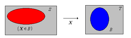
The Distribution of a Random Variable

Suppose now that \(X\) is a random variable for the experiment, taking values in a set \(T\). Recall that mathematically, \( X \) is a function from \( S \) into \( T \), and \( \{X \in B\}\) denotes the event \(\{s \in S: X(s) \in B\} \) for \( B \subseteq T \). Intuitively, \( X \) is a variable of interest for the experiment, and every meaningful statement about \( X \) defines an event.

The function \(B \mapsto \P(X \in B)\) for \( B \subseteq T \) defines a probability measure on \(T\).

Proof

Figure \(\PageIndex{2}\): A set \( B \in \mathscr T \) corresponds to the event \( \{X \in B\} \in \mathscr S \)

The probability measure in (5) is called the probability distribution of \(X\), so we have all of the ingredients for a new probability space.

A random variable \(X\) with values in \( T \) defines a new probability space:

1. \(T\) is the set of outcomes.
2. Subsets of \( T \) are the events.
3. The probability distribution of \(X\) is the probability measure on \( T \).

This probability space corresponds to the new random experiment in which the outcome is \( X \). Moreover, recall that the outcome of the experiment itself can be thought of as a random variable. Specifically, if we let \(T = S\) we let \(X\) be the identity function on \(S\), so that \( X(s) = s \) for \( s \in S \). Then \(X\) is a random variable with values in \( S \) and \(\P(X \in A) = \P(A)\) for each event \( A \). Thus, every probability measure can be thought of as the distribution of a random variable.

Constructions

Measures

How can we construct probability measures? As noted briefly above, there are other measures of the size of sets; in many cases, these can be converted into probability measures. First, a positive measure \(\mu\) on the sample space \((S, \mathscr S)\) is a real-valued function defined on \(\mathscr{S}\) that satisfies axioms (a) and (c) in (1), and then \( (S, \mathscr S, \mu) \) is a measure space. In general, \(\mu(A)\) is allowed to be infinite. However, if \(\mu(S)\) is positive and finite (so that \( \mu \) is a finite positive measure), then \(\mu\) can easily be re-scaled into a probability measure.

If \(\mu\) is a positive measure on \(S\) with \(0 \lt \mu(S) \lt \infty\) then \(\P\) defined below is a probability measure. \[\P(A) = \frac{\mu(A)}{\mu(S)}, \quad A \in \mathscr S\]

Proof

1. \(\P(A) \ge 0\) since \(\mu(A) \ge 0\) and \(0 \lt \mu(S) \lt \infty\).
2. \(\P(S) = \mu(S) \big/ \mu(S) = 1\)
3. If \(\{A_i: i \in I\}\) is a countable collection of disjoint events then \[ \P\left(\bigcup_{i \in I} A_i \right) = \frac{1}{\mu(S)} \mu\left(\bigcup_{i \in I} A_i \right) = \frac{1}{\mu(S)} \sum_{i \in I} \mu(A_i) = \sum_{i \in I} \frac{\mu(A_i)}{\mu(S)} = \sum_{i \in I} \P(A_i) \]

In this context, \(\mu(S)\) is called the normalizing constant. In the next two subsections, we consider some very important special cases.

Discrete Distributions

In this discussion, we assume that the sample space \((S, \mathscr S)\) is discrete. Recall that this means that the set of outcomes \(S\) is countable and that \(\mathscr S = \mathscr P(S)\) is the collection of all subsets of \(S\), so that every subset is an event. The standard measure on a discrete space is counting measure \(\#\), so that \(\#(A)\) is the number of elements in \(A\) for \(A \subseteq S\). When \( S \) is finite, the probability measure corresponding to counting measure as constructed in above is particularly important in combinatorial and sampling experiments.

Suppose that \(S\) is a finite, nonempty set. The discrete uniform distribution on \(S\) is given by \[\P(A) = \frac{\#(A)}{\#(S)}, \quad A \subseteq S\]

The underlying model is refereed to as the classical probability model, because historically the very first problems in probability (involving coins and dice) fit this model.

In the general discrete case, if \(\P\) is a probability measure on \(S\), then since \( S \) is countable, it follows from countable additivity that \(\P\) is completely determined by its values on the singleton events. Specifically, if we define \(f(x) = \P\left(\{x\}\right)\) for \(x \in S\), then \(\P(A) = \sum_{x \in A} f(x)\) for every \(A \subseteq S\). By axiom (a), \(f(x) \ge 0\) for \(x \in S\) and by axiom (b), \(\sum_{x \in S} f(x) = 1\). Conversely, we can give a general construction for defining a probability measure on a discrete space.

Suppose that \( g: S \to [0, \infty) \). Then \(\mu\) defined by \( \mu(A) = \sum_{x \in A} g(x) \) for \( A \subseteq S \) is a positive measure on \(S\). If \(0 \lt \mu(S) \lt \infty\) then \(\P\) defined as follows is a probability measure on \(S\). \[ \P(A) = \frac{\mu(A)}{\mu(S)} = \frac{\sum_{x \in A} g(x)}{\sum_{x \in S} g(x)}, \quad A \subseteq S\]

Proof

Trivially \(\mu(A) \ge 0\) for \( A \subseteq S \) since \(g\) is nonnegative. The countable additivity property holds since the terms in a sum of nonnegative numbers can be rearranged in any way without altering the sum. Thus let \(\{A_i: i \in I\}\) be a countable collection of disjoint subsets of \( S \), and let \(A = \bigcup_{i \in I} A_i\) then \[ \mu(A) = \sum_{x \in A} g(x) = \sum_{i \in I} \sum_{x \in A_i} g(x) = \sum_{i \in I} \mu(A_i) \] If \( 0 \lt \mu(S) \lt \infty \) then \( \P \) is a probability measure by scaling result above.

In the context of our previous remarks, \(f(x) = g(x) \big/ \mu(S) = g(x) \big/ \sum_{y \in S} g(y)\) for \( x \in S \). Distributions of this type are said to be discrete. Discrete distributions are studied in detail in the chapter on Distributions.

If \(S\) is finite and \(g\) is a constant function, then the probability measure \(\P\) associated with \( g \) is the discrete uniform distribution on \(S\).

Proof

Suppose that \(g(x) = c\) for \(x \in S\) where \(c \gt 0\). Then \(\mu(A) = c \#(A) \) and hence \(\P(A) = \mu(A) \big/ \mu(S) = \#(A) \big/ \#(S)\) for \( A \subseteq S \).

Continuous Distributions

The probability distributions that we will construct next are continuous distributions on \( \R^n \) for \( n \in \N_+ \) and require some calculus.

For \(n \in \N_+\), the standard measure \( \lambda_n \) on \( \R^n \) is given by \[\lambda_n(A) = \int_A 1 \, dx, \quad A \subseteq \R^n\] In particular, \( \lambda_1(A) \) is the length of ( A \subseteq \R \), \( lambda_2(A) \) is the area of \( A \subseteq \R^2 \), and \( \lambda_3(A) \) is the volume of \( A \subseteq \R^3 \).

Details

Technically, \( \lambda_n \) is Lebesgue measure on the measurable subsets of \( \R^n \), named for Henri Lebesgue. The representation above in terms of the ordinary Riemann integral of calculus is valid for the subsets that typically occur in applications. As usual, all subsets of \( \R^n \) in the discussion below are assumed to be mearuable.

When \(n \gt 3\), \(\lambda_n(A)\) is sometimes called the \(n\)-dimensional volume of \(A \subseteq \R_n\). The probability measure associated with \( \lambda_n \) on a set with positive, finite \( n \)-dimensional volume is particularly important.

Suppose that \(S \subseteq \R_n\) with \(0 \lt \lambda_n(S) \lt \infty\). The continuous uniform distribution on \( S \) is defined by \[\P(A) = \frac{\lambda_n(A)}{\lambda_n(S)}, \quad A \subseteq S\]

Note that the continuous uniform distribution is analogous to the discrete uniform distribution defined in (8), but with Lebesgue measure \( \lambda_n \) replacing counting measure \( \# \). We can generalize this construction to produce many other distributions.

Suppose again that \( S \subseteq \R^n\) and that \( g: S \to [0, \infty) \). Then \( \mu \) defined by \( \mu(A) = \int_A g(x) \, dx \) for \( A \subseteq S \) is a positive measure on \( S \). If \(0 \lt \mu(S) \lt \infty\), then \( \P \) defined as follows is a probability measure on \( S \). \[\P(A) = \frac{\mu(A)}{\mu(S)} = \frac{\int_A g(x) \, dx}{\int_S g(x) \, dx}, \quad A \in \mathscr S\]

Proof

Technically, the integral in the definition of \(\mu(A)\) is the Lebesgue integral, but this integral agrees with the ordinary Riemann integral of calculus when \(g\) and \(A\) are sufficiently nice. The function \(g\) is assumed to be measurable and is the density function of \(\mu\) with respect to \(\lambda_n\). Technicalities aside, the proof is straightforward:

1. \( \mu(A) \ge 0 \) for \( A \subseteq S \) since \( g \) is nonnegative.
2. If \(\{A_i: i \in I\}\) is a countable disjoint collection of subsets of \(S\) and \(A = \bigcup_{i \in I} A_i\), then by a basic property of the integral, \[\mu(A) = \int_A g(x) \, dx = \sum_{i \in I} \int_{A_i} g(x) \, dx = \sum_{i \in I} \mu(A_i)\]

If \( 0 \lt \mu(S) \lt \infty \) then \( \P \) is a probability measure on \( S \) by the scaling result above.

Distributions of this type are said to be continuous. Continuous distributions are studied in detail in the chapter on Distributions. Note that the continuous distribution above is analogous to the discrete distribution in (9), but with integrals replacing sums. The general theory of integration allows us to unify these two special cases, and many others besides.

Rules of Probability

Basic Rules

Suppose again that we have a random experiment modeled by a probability space \( (S, \mathscr S, \P) \), so that \(S\) is the set of outcomes, \( \mathscr S \) the collection of events, and \( \P \) the probability measure. In the following theorems, \(A\) and \(B\) are events. The results follow easily from the axioms of probability in (1), so be sure to try the proofs yourself before reading the ones in the text.

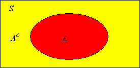
\(\P(A^c) = 1 - \P(A)\). This is known as the complement rule.

Proof

Figure \(\PageIndex{3}\): The complement rule

\(\P(\emptyset) = 0\).

Proof

This follows from the the complement rule applied to \(A = S\).

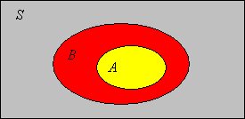
\(\P(B \setminus A) = \P(B) - \P(A \cap B)\). This is known as the difference rule.

Proof

Figure \(\PageIndex{4}\): The difference rule

If \(A \subseteq B\) then \(\P(B \setminus A) = \P(B) - \P(A)\).

Proof

This result is a corollary of the difference rule. Note that \(A \cap B = A\).

Recall that if \( A \subseteq B \) we sometimes write \( B - A \) for the set difference, rather than \( B \setminus A \). With this notation, the difference rule has the nice form \( \P(B - A) = \P(B) - \P(A) \).

If \(A \subseteq B\) then \(\P(A) \le \P(B)\).

Proof

This result is a corollary of the previous result. Note that \( \P(B \setminus A) \ge 0 \) and hence \( \P(B) - \P(A) \ge 0 \).

Thus, \(\P\) is an increasing function, relative to the subset partial order on the collection of events \( \mathscr S \), and the ordinary order on \(\R\). In particular, it follows that \(\P(A) \le 1\) for any event \(A\).

Figure \(\PageIndex{5}\): The increasing property

Suppose that \(A \subseteq B\).

1. If \(\P(B) = 0\) then \(\P(A) = 0\).
2. If \(\P(A) = 1\) then \(\P(B) = 1\).

Proof

This follows immediately from the increasing property in the last theorem.

The Boole and Bonferroni Inequalities

The next result is known as Boole's inequality, named after George Boole. The inequality gives a simple upper bound on the probability of a union.

If \(\{A_i: i \in I\}\) is a countable collection of events then \[\P\left( \bigcup_{i \in I} A_i \right) \le \sum_{i \in I} \P(A_i)\]

Proof

Figure \(\PageIndex{6}\): Boole's inequality

Intuitively, Boole's inequality holds because parts of the union have been measured more than once in the sum of the probabilities on the right. Of course, the sum of the probabilities may be greater than 1, in which case Boole's inequality is not helpful. The following result is a simple consequence of Boole's inequality.

If \(\{A_i: i \in I\}\) is a countable collection of events with \(\P(A_i) = 0\) for each \(i \in I\), then \[\P\left( \bigcup_{i \in I} A_i \right) = 0\]

An event \(A\) with \(\P(A) = 0\) is said to be null. Thus, a countable union of null events is still a null event.

The next result is known as Bonferroni's inequality, named after Carlo Bonferroni. The inequality gives a simple lower bound for the probability of an intersection.

If \(\{A_i: i \in I\}\) is a countable collection of events then \[\P\left( \bigcap_{i \in I} A_i \right) \ge 1 - \sum_{i \in I}\left[1 - \P(A_i)\right]\]

Proof

By De Morgan's law, \( \left(\bigcap_{i \in I} A_i\right)^c = \bigcup_{i \in I} A_i^c \). Hence by Boole's inequality, \[ \P\left[\left(\bigcap_{i \in I} A_i\right)^c\right] \le \sum_{i \in I} \P(A_i^c) = \sum_{i \in I} \left[1 - \P(A_i)\right] \] Using the complement rule again gives Bonferroni's inequality.

Of course, the lower bound in Bonferroni's inequality may be less than or equal to 0, in which case it's not helpful. The following result is a simple consequence of Bonferroni's inequality.

If \(\{A_i: i \in I\}\) is a countable collection of events with \(\P(A_i) = 1\) for each \(i \in I\), then \[\P\left( \bigcap_{i \in I} A_i \right) = 1\]

An event \(A\) with \(\P(A) = 1\) is sometimes called almost sure or almost certain. Thus, a countable intersection of almost sure events is still almost sure.

Suppose that \(A\) and \(B\) are events in an experiment.

1. If \(\P(A) = 0\), then \(\P(A \cup B) = \P(B)\).
2. If \(\P(A) = 1\), then \(\P(A \cap B) = \P(B)\).

Proof

1. Using the increasing property and Boole's inequality we have \( \P(B) \le \P(A \cup B) \le \P(A) + \P(B) = \P(B) \)
2. Using the increasing property and Bonferonni's inequality we have \( \P(B) = \P(A) + \P(B) - 1 \le \P(A \cap B) \le P(B) \)

The Partition Rule

Suppose that \(\{A_i: i \in I\}\) is a countable collection of events that partition \(S\). Recall that this means that the events are disjoint and their union is \(S\). For any event \(B\), \[\P(B) = \sum_{i \in I} \P(A_i \cap B)\]

Proof

Figure \(\PageIndex{7}\): The partition rule

Naturally, this result is useful when the probabilities of the intersections are known. Partitions usually arise in connection with a random variable. Suppose that \(X\) is a random variable taking values in a countable set \(T\), and that \(B\) is an event. Then \[\P(B) = \sum_{x \in T} \P(X = x, B)\] In this formula, note that the comma acts like the intersection symbol in the previous formula.

The Inclusion-Exclusion Rule

The inclusion-exclusion formulas provide a method for computing the probability of a union of events in terms of the probabilities of the various intersections of the events. The formula is useful because often the probabilities of the intersections are easier to compute. Interestingly, however, the same formula works for computing the probability of an intersection of events in terms of the probabilities of the various unions of the events. This version is rarely stated, because it's simply not that useful. We start with two events.

If \( A, \, B \) are events thatn \(\P(A \cup B) = \P(A) + \P(B) - \P(A \cap B)\).

Proof

Figure \(\PageIndex{8}\): The probability of the union of two events

Here is the complementary result for the intersection in terms of unions:

If \( A, \, B \) are events then \(\P(A \cap B) = \P(A) + \P(B) - \P(A \cup B)\).

Proof

This follows immediately from the previous formula be rearranging the terms

Next we consider three events.

If \( A, \, B, \, C \) are events then \(\P(A \cup B \cup C) = \P(A) + \P(B) + \P(C) - \P(A \cap B) - \P(A \cap C) - \P(B \cap C) + \P(A \cap B \cap C)\).

Analytic Proof

First note that \( A \cup B \cup C = (A \cup B) \cup [C \setminus (A \cup B)] \). The event in parentheses and the event in square brackets are disjoint. Thus, using the additivity axiom and the difference rule, \[ \P(A \cup B \cup C) = \P(A \cup B) + \P(C) - \P\left[C \cap (A \cup B)\right] = \P(A \cup B) + \P(C) - \P\left[(C \cap A) \cup (C \cap B)\right] \] Using the inclusion-exclusion rule for two events (twice) we have \[ \P(A \cup B \cup C) = \P(A) + \P(B) - \P(A \cap B) + \P(C) - \left[\P(C \cap A) + \P(C \cap B) - \P(A \cap B \cap C)\right] \]

Proof by accounting

Figure \(\PageIndex{8}\): The probability of the union of three events

Here is the complementary result for the probability of an intersection in terms of the probabilities of the unions:

If \( A, \, B, \, C \) are events then \(\P(A \cap B \cap C) = \P(A) + \P(B) + \P(C) - \P(A \cup B) - \P(A \cup C) - \P(B \cup C) + \P(A \cup B \cup C)\).

Proof

This follows from solving for \( \P(A \cap B \cap C) \) in the previous result, and then using the result for two events on \( \P(A \cap B) \), \( \P(B \cap C) \), and \( \P(A \cap C) \).

The inclusion-exclusion formulas for two and three events can be generalized to \(n\) events. For the remainder of this discussion, suppose that \( \{A_i: i \in I\} \) is a collection of events where \( I \) is an index set with \( \#(I) = n \).

The general inclusion-exclusion formula for the probability of a union. \[\P\left( \bigcup_{i \in I} A_i \right) = \sum_{k = 1}^n (-1)^{k - 1} \sum_{J \subseteq I, \; \#(J) = k} \P\left( \bigcap_{j \in J} A_j \right)\]

Proof by induction

The proof is by induction on \(n\). We have already established the formula for \( n = 2 \) and \( n = 3 \). Thus, suppose that the inclusion-exclusion formula holds for a given \( n \), and suppose that \( (A_1, A_2, \ldots, A_{n+1}) \) is a sequence of \( n + 1 \) events. Then \[ \bigcup_{i=1}^{n + 1} A_i = \left(\bigcup_{i=1}^n A_i \right) \cup \left[ A_{n+1} \setminus \left(\bigcup_{i=1}^n A_i\right) \right] \] As before, the event in parentheses and the event in square brackets are disjoint. Thus using the additivity axiom, the difference rule, and the distributive rule we have \[ \P\left(\bigcup_{i=1}^{n+1} A_i\right) = \P\left(\bigcup_{i=1}^n A_i\right) + \P(A_{n+1}) - \P\left(\bigcup_{i=1}^n (A_{n+1} \cap A_i) \right) \] By the induction hypothesis, the inclusion-exclusion formula holds for each union of \( n \) events on the right. Applying the formula and simplifying gives the inclusion-exclusion formula for \( n + 1 \) events.

Proof by accounting

This is the general version of the same argument we used above for 3 events. \( \bigcup_{i \in I} A_i \) is the union of the disjoint events of the form \( \left(\bigcap_{i \in K} A_i\right) \cap \left(\bigcap_{i \in K^c} A_i\right)\) where \( K \) is a nonempty subset of the index set \( I \). In the inclusion-exclusion formula, the event corresponding to a given \( K \) is measured in \( \P\left(\bigcap_{j \in J} A_j\right) \) for every nonempty \( J \subseteq K \). Suppose that \( \#(K) = k \). Accounting for the positive and negative signs, the net measurement is \( \sum_{j=1}^k (-1)^{j-1} \binom{k}{j} = 1 \).

Here is the complementary result for the probability of an intersection in terms of the probabilities of the various unions:

The general inclusion-exclusion formula for the probability of an intersection. \[\P\left( \bigcap_{i \in I} A_i \right) = \sum_{k = 1}^n (-1)^{k - 1} \sum_{J \subseteq I, \; \#(J) = k} \P\left( \bigcup_{j \in J} A_j \right)\]

The general inclusion-exclusion formulas are not worth remembering in detail, but only in pattern. For the probability of a union, we start with the sum of the probabilities of the events, then subtract the probabilities of all of the paired intersections, then add the probabilities of the third-order intersections, and so forth, alternating signs, until we get to the probability of the intersection of all of the events.

The general Bonferroni inequalities (for a union) state that if sum on the right in the general inclusion-exclusion formula is truncated, then the truncated sum is an upper bound or a lower bound for the probability on the left, depending on whether the last term has a positive or negative sign. Here is the result stated explicitly:

Suppose that \( m \in \{1, 2, \ldots, n - 1\} \). Then

1. \(\P\left( \bigcup_{i \in I} A_i \right) \le \sum_{k = 1}^m (-1)^{k - 1} \sum_{J \subseteq I, \; \#(J) = k} \P\left( \bigcap_{j \in J} A_j \right)\) if \( m \) is odd.
2. \(\P\left( \bigcup_{i \in I} A_i \right) \ge \sum_{k = 1}^m (-1)^{k - 1} \sum_{J \subseteq I, \; \#(J) = k} \P\left( \bigcap_{j \in J} A_j \right)\) if \( m \) is event.

Proof

Let \( P_k = \sum_{J \subseteq I, \; \#(J) = k} \P\left( \bigcap_{j \in J} A_j \right) \), the absolute value of the \( k \)th term in the inclusion-exclusion formula. The result follows since the inclusion-exclusion formula is an alternating series, and \( P_k \) is decreasing in \( k \).

More elegant proofs of the inclusion-exclusion formula and the Bonferroni inequalities can be constructed using expected value.

Note that there is a probability term in the inclusion-exclusion formulas for every nonempty subset \( J \) of the index set \( I \), with either a positive or negative sign, and hence there are \( 2^n - 1 \) such terms. These probabilities suffice to compute the probability of any event that can be constructed from the given events, not just the union or the intersection.

The probability of any event that can be constructed from \( \{A_i: i \in I\} \) can be computed from either of the following collections of \( 2^n - 1 \) probabilities:

1. \( \P\left(\bigcap_{j \in J} A_j\right) \) where \( J \) is a nonempty subset of \( I \).
2. \( \P\left(\bigcup_{j \in J} A_j\right) \) where \( J \) is a nonempty subset of \( I \).

Remark

If you go back and look at your proofs of the rules of probability above, you will see that they hold for any finite measure \(\mu\), not just probability. The only change is that the number 1 is replaced by \(\mu(S)\). In particular, the inclusion-exclusion rule is as important in combinatorics (the study of counting measure) as it is in probability.

Examples and Applications

Probability Rules

Suppose that \(A\) and \(B\) are events in an experiment with \(\P(A) = \frac{1}{3}\), \(\P(B) = \frac{1}{4}\), \(\P(A \cap B) = \frac{1}{10}\). Express each of the following events in the language of the experiment and find its probability:

1. \(A \setminus B\)
2. \(A \cup B\)
3. \(A^c \cup B^c\)
4. \(A^c \cap B^c\)
5. \(A \cup B^c\)

Answer

1. \(A\) occurs but not \(B\). \(\frac{7}{30}\)
2. \(A\) or \(B\) occurs. \(\frac{29}{60}\)
3. One of the events does not occur. \(\frac{9}{10}\)
4. Neither event occurs. \(\frac{31}{60}\)
5. Either \(A\) occurs or \(B\) does not occur. \(\frac{17}{20}\)

Suppose that \(A\), \(B\), and \(C\) are events in an experiment with \(\P(A) = 0.3\), \(\P(B) = 0.2\), \(\P(C) = 0.4\), \(\P(A \cap B) = 0.04\), \(\P(A \cap C) = 0.1\), \(\P(B \cap C) = 0.1\), \(\P(A \cap B \cap C) = 0.01\). Express each of the following events in set notation and find its probability:

1. At least one of the three events occurs.
2. None of the three events occurs.
3. Exactly one of the three events occurs.
4. Exactly two of the three events occur.

Answer

1. \(\P(A \cup B \cup C) = 0.67\)
2. \(\P[(A \cup B \cup C)^c] = 0.37\)
3. \(\P[(A \cap B^c \cap C^c) \cup (A^c \cap B \cap C^c) \cup (A^c \cap B^c \cap C)] = 0.45\)
4. \(\P[(A \cap B \cap C^c) \cup (A \cap B^c \cap C) \cup (A^c \cap B \cap C)] = 0.21\)

Suppose that \(A\) and \(B\) are events in an experiment with \(\P(A \setminus B) = \frac{1}{6}\), \(\P(B \setminus A) = \frac{1}{4}\), and \(\P(A \cap B) = \frac{1}{12}\). Find the probability of each of the following events:

1. \(A\)
2. \(B\)
3. \(A \cup B\)
4. \(A^c \cup B^c\)
5. \(A^c \cap B^c\)

Answer

1. \(\frac{1}{4}\)
2. \(\frac{1}{3}\)
3. \(\frac{1}{2}\)
4. \(\frac{11}{12}\)
5. \(\frac{1}{2}\)

Suppose that \(A\) and \(B\) are events in an experiment with \(\P(A) = \frac{2}{5}\), \(\P(A \cup B) = \frac{7}{10}\), and \(\P(A \cap B) = \frac{1}{6}\). Find the probability of each of the following events:

1. \(B\)
2. \(A \setminus B\)
3. \(B \setminus A\)
4. \(A^c \cup B^c\)
5. \(A^c \cap B^c\)

Answer

1. \(\frac{7}{15}\)
2. \(\frac{7}{30}\)
3. \(\frac{3}{10}\)
4. \(\frac{5}{6}\)
5. \(\frac{3}{10}\)

Suppose that \(A\), \(B\), and \(C\) are events in an experiment with \(\P(A) = \frac{1}{3}\), \(\P(B) = \frac{1}{4}\), \(\P(C) = \frac{1}{5}\).

1. Use Boole's inequality to find an upper bound for \(\P(A \cup B \cup C)\).
2. Use Bonferronis's inequality to find a lower bound for \(\P(A \cap B \cap C)\).

Answer

1. \(\frac{47}{60}\)
2. \(-\frac{83}{60}\), not helpful.

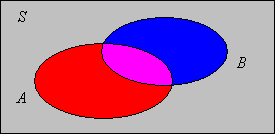
Open the simple probability experiment.

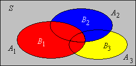
1. Note the 16 events that can be constructed from \( A \) and \( B \) using the set operations of union, intersection, and complement.
2. Given \( \P(A) \), \( \P(B) \), and \( \P(A \cap B) \) in the table, use the rules of probability to verify the probabilities of the other events.
3. Run the experiment 1000 times and compare the relative frequencies of the events with the probabilities of the events.

Suppose that \(A\), \(B\), and \(C\) are events in a random experiment with \( \P(A) = 1/4 \), \( \P(B) = 1/3 \), \( \P(C) = 1/6 \), \( \P(A \cap B) = 1/18 \), \( \P(A \cap C) = 1/16 \), \( \P(B \cap C) = 1/12 \), and \( \P(A \cap B \cap C) = 1/24 \). Find the probabilities of the various unions:

1. \( A \cup B \)
2. \( A \cup C \)
3. \( B \cup C \)
4. \( A \cup B \cup C \)

Answer

1. \( 19/36 \)
2. \( 17/48 \)
3. \( 5/12 \)
4. \( 85/144 \)

Suppose that \(A\), \(B\), and \(C \) are events in a random experiment with \( \P(A) = 1/4 \), \( \P(B) = 1/4 \), \( \P(C) = 5/16 \), \( \P(A \cup B) = 7/16 \), \( \P(A \cup C) = 23/48 \), \( \P(B \cup C) = 11/24 \), and \( \P(A \cup B \cup C) = 7/12 \). Find the probabilities of the various intersections:

1. \( A \cap B \)
2. \( A \cap C \)
3. \( B \cap C \)
4. \( A \cap B \cap C \)

Answer

1. \( 1/16 \)
2. \( 1/12 \)
3. \( 5/48 \)
4. \( 1/48 \)

Suppose that \(A\), \(B\), and \(C\) are events in a random experiment. Explicitly give all of the Bonferroni inequalities for \( \P(A \cup B \cup C) \)

Proof

1. \( \P(A \cup B \cup C) \le \P(A) + \P(B) + \P(C) \)
2. \( \P(A \cup B \cup C) \ge \P(A) + \P(B) + \P(C) - \P(A \cap B) - \P(A \cap C) - \P(B \cap C) \)
3. \( \P(A \cup B \cup C) = \P(A) + \P(B) + \P(C) - \P(A \cap B) - \P(A \cap C) - \P(B \cap C) + \P(A \cap B \cap C)\)

Coins

Consider the random experiment of tossing a coin \(n\) times and recording the sequence of scores \(\bs{X} = (X_1, X_2, \ldots, X_n)\) (where 1 denotes heads and 0 denotes tails). This experiment is a generic example of \(n\) Bernoulli trials, named for Jacob Bernoulli. Note that the set of outcomes is \(S = \{0, 1\}^n\), the set of bit strings of length \(n\). If the coin is fair, then presumably, by the very meaning of the word, we have no reason to prefer one point in \(S\) over another. Thus, as a modeling assumption, it seems reasonable to give \(S\) the uniform probability distribution in which all outcomes are equally likely.

Suppose that a fair coin is tossed 3 times and the sequence of coin scores is recorded. Let \(A\) be the event that the first coin is heads and \(B\) the event that there are exactly 2 heads. Give each of the following events in list form, and then compute the probability of the event:

1. \(A\)
2. \(B\)
3. \(A \cap B\)
4. \(A \cup B\)
5. \(A^c \cup B^c\)
6. \(A^c \cap B^c\)
7. \(A \cup B^c\)

Answer

1. \(\{100, 101, 110, 111\}\), \(\frac{1}{2}\)
2. \(\{110, 101, 011\}\), \(\frac{3}{8}\)
3. \(\{110, 101\}\), \(\frac{1}{4}\)
4. \(\{100, 101, 110, 111, 011\}\), \(\frac{5}{8}\)
5. \(\{000, 001, 010, 100, 011, 111\}\), \(\frac{3}{4}\)
6. \(\{000, 001, 010\}\), \(\frac{3}{8}\)
7. \(\{100, 101, 110, 111, 000, 010, 001\}\), \(\frac{7}{8}\)

In the Coin experiment, select 3 coins. Run the experiment 1000 times, updating after every run, and compute the empirical probability of each event in the previous exercise.

Suppose that a fair coin is tossed 4 times and the sequence of scores is recorded. Let \(Y\) denote the number of heads. Give the event \(\{Y = k\}\) (as a subset of the sample space) in list form, for each \(k \in \{0, 1, 2, 3, 4\}\), and then give the probability of the event.

Answer

1. \(\{Y = 0\} = \{0000\}\), \(\P(Y = 0) = \frac{1}{16}\)
2. \(\{Y = 1\} = \{1000, 0100, 0010, 0001\}\), \(\P(Y = 1) = \frac{4}{16}\)
3. \(\{Y = 2\} = \{1100, 1010, 1001, 0110, 0101, 0011\}\), \(\P(Y = 2) = \frac{6}{16}\)
4. \(\{Y = 3\} = \{1110, 1101, 1011, 0111\}\), \(\P(Y = 3) = \frac{4}{16}\)
5. \(\{Y = 4\} = \{1111\}\), \(\P(Y = 4) = \frac{1}{16}\)

Suppose that a fair coin is tossed \(n\) times and the sequence of scores is recorded. Let \(Y\) denote the number of heads.

\[\P(Y = k) = \binom{n}{k} \left( \frac{1}{2} \right)^n, \quad k \in \{0, 1, \ldots, n\}\]

Proof

The number of bit strings of length \(n\) is \(2^n\), and since the coin is fair, these are equally likely. The number of bit strings of length \(n\) with exactly \(k\) 1's is \(\binom{n}{k}\). Hence the probability of 1 occurring exactly \(k\) times is \(\binom{n}{k} \big/ 2^n\).

The distribution of \(Y\) in the last exercise is a special case of the binomial distribution. The binomial distribution is studied in more detail in the chapter on Bernoulli Trials.

Dice

Consider the experiment of throwing \(n\) distinct, \(k\)-sided dice (with faces numbered from 1 to \(k\)) and recording the sequence of scores \(\bs{X} = (X_1, X_2, \ldots, X_n)\). We can record the outcome as a sequence because of the assumption that the dice are distinct; you can think of the dice as somehow labeled from 1 to \(n\), or perhaps with different colors. The special case \(k = 6\) corresponds to standard dice. In general, note that the set of outcomes is \(S = \{1, 2, \ldots, k\}^n\). If the dice are fair, then again, by the very meaning of the word, we have no reason to prefer one point in \( S \) over another, so as a modeling assumption it seems reasonable to give \(S\) the uniform probability distribution.

Suppose that two fair, standard dice are thrown and the sequence of scores recorded. Let \(A\) denote the event that the first die score is less than 3 and \(B\) the event that the sum of the dice scores is 6. Give each of the following events in list form and then find the probability of the event.

1. \(A\)
2. \(B\)
3. \(A \cap B\)
4. \(A \cup B\)
5. \(B \setminus A\)

Answer

1. \(\{(1,1),(1,2),(1,3),(1,4),(1,5),(1,6),(2,1),(2,2),(2,3),(2,4),(2,5),(2,6)\}\), \(\frac{12}{36}\)
2. \(\{(1,5),(5,1),(2,4),(4,2),(3,3)\}\), \(\frac{5}{36}\)
3. \(\{(1,5), (2,4)\}\), \(\frac{2}{36}\)
4. \(\{(1,1),(1,2),(1,3),(1,4),(1,5),(1,6),(2,1),(2,2),(2,3),(2,4),(2,5),(2,6),(5,1),(4,2),(3,3)\}\), \(\frac{15}{36}\)
5. \(\{(5,1), (4,2), (3,3)\}\), \(\frac{3}{36}\)

In the dice experiment, set \(n = 2\). Run the experiment 100 times and compute the empirical probability of each event in the previous exercise.

Consider again the dice experiment with \(n = 2\) fair dice. Let \( S \) denote the set of outcomes, \(Y\) the sum of the scores, \(U\) the minimum score, and \(V\) the maximum score.

1. Express \(Y\) as a function on \( S \) and give the set of values.
2. Find \(\P(Y = y)\) for each \(y\) in the set in part (a).
3. Express \(U\) as a function on \( S \) and give the set of values.
4. Find \(\P(U = u)\) for each \(u\) in the set in part (c).
5. Express \(V\) as a function on \( S \) and give the set of values.
6. Find \(\P(V = v)\) for each \(v\) in the set in part (e).
7. Find the set of values of \((U, V)\).
8. Find \(\P(U = u, V = v)\) for each \((u, v)\) in the set in part (g).

Answer

Note that \( S = \{1, 2, 3, 4, 5, 6\}^2 \).

1. \(Y(x_1, x_2) = x_1 + x_2\) for \( (x_1, x_2) \in S \). The set of values is \(\{2, 3, \ldots, 12\}\)

2. \(y\)	2	3	4	5	6	7	8	9	10	11	12
   \(\P(Y = y)\)	\(\frac{1}{36}\)	\(\frac{2}{36}\)	\(\frac{3}{36}\)	\(\frac{4}{36}\)	\(\frac{5}{36}\)	\(\frac{6}{36}\)	\(\frac{5}{36}\)	\(\frac{4}{36}\)	\(\frac{3}{36}\)	\(\frac{2}{36}\)	\(\frac{1}{36}\)

3. \(U(x_1, x_2) = \min\{x_1, x_2\}\) for \( (x_1, x_2) \in S \). The set of values is \(\{1, 2, 3, 4, 5, 6\}\)

4. \(u\)	1	2	3	4	5	6
   \(\P(U = u)\)	\(\frac{11}{36}\)	\(\frac{9}{36}\)	\(\frac{7}{36}\)	\(\frac{5}{36}\)	\(\frac{3}{36}\)	\(\frac{1}{36}\)

5. \(V(x_1, x_2) = \max\{x_1, x_2\}\) for \( (x_1, x_2) \in S \). The set of values is \(\{1, 2, 3, 4, 5, 6\}\)

6. \(v\)	1	2	3	4	5	6
   \(\P(V = v)\)	\(\frac{1}{36}\)	\(\frac{3}{36}\)	\(\frac{5}{36}\)	\(\frac{7}{36}\)	\(\frac{9}{36}\)	\(\frac{11}{36}\)

7. \(\left\{(u, v) \in S: u \le v\right\}\)
8. \(\P(U = u, V = v) = \begin{cases} \frac{2}{36}, & u \lt v \\ \frac{1}{36}, & u = v \end{cases}\)

In the previous exercise, note that \((U, V)\) could serve as the outcome vector for the experiment of rolling two standard, fair dice if we do not bother to distinguish the dice (so that we might as well record the smaller score first and then the larger score). Note that this random vector does not have a uniform distribution. On the other hand, we might have chosen at the beginning to just record the unordered set of scores and, as a modeling assumption, imposed the uniform distribution on the corresponding set of outcomes. Both models cannot be right, so which model (if either) describes real dice in the real world? It turns out that for real (fair) dice, the ordered sequence of scores is uniformly distributed, so real dice behave as distinct objects, whether you can tell them apart or not. In the early history of probability, gamblers sometimes got the wrong answers for events involving dice because they mistakenly applied the uniform distribution to the set of unordered scores. It's an important moral. If we are to impose the uniform distribution on a sample space, we need to make sure that it's the right sample space.

A pair of fair, standard dice are thrown repeatedly until the sum of the scores is either 5 or 7. Let \(A\) denote the event that the sum of the scores on the last throw is 5 rather than 7. Events of this type are important in the game of craps.

1. Suppose that we record the pair of scores on each throw. Give the set of outcomes \(S\) and express \(A\) as a subset of \(S\).
2. Compute the probability of \(A\) in the setting of part (a).
3. Now suppose that we just record the pair of scores on the last throw. Give the set of outcomes \(T\) and express \(A\) as a subset of \(T\).
4. Compute the probability of \(A\) in the setting of parts (c).

Answer

Let \(D_5 = \{(1,4), (2,3), (3,2), (4,1)\}\), \(D_7 = \{(1,6), (2,5), (3,4), (4,3), (5,2), (6,1)\}\), \(D = D_5 \cup D_7\), \(C = \{1, 2, 3, 4, 5, 6\}^2 \setminus D\)

1. \(S = D \cup (C \times D) \cup (C^2 \times D) \cup \cdots\), \(A = D_5 \cup (C \times D_5) \cup (C^2 \times D_5) \cup \cdots\)
2. \(\frac{2}{5}\)
3. \(T = D\), \(A = D_5\)
4. \(\frac{2}{5}\)

The previous problem shows the importance of defining the set of outcomes appropriately. Sometimes a clever choice of this set (and appropriate modeling assumptions) can turn a difficult problem into an easy one.

Sampling Models

Recall that many random experiments can be thought of as sampling experiments. For the general finite sampling model, we start with a population \(D\) with \(m\) (distinct) objects. We select a sample of \(n\) objects from the population, so that the sample space \(S\) is the set of possible samples. If we select a sample at random then the outcome \(\bs{X}\) (the random sample) is uniformly distributed on \(S\): \[\P(\bs{X} \in A) = \frac{\#(A)}{\#(S)}, \quad A \subseteq S\] Recall from the section on Combinatorial Structures that there are four common types of sampling from a finite population, based on the criteria of order and replacement.

• If the sampling is with replacement and with regard to order, then the set of samples is the Cartesian power \(D^n\). The number of samples is \(m^n\).
• If the sampling is without replacement and with regard to order, then the set of samples is the set of all permutations of size \(n\) from \(D\). The number of samples is \(m^{(n)} = m (m - 1) \cdots (m - n + 1)\).
• If the sampling is without replacement and without regard to order, then the set of samples is the set of all combinations (or subsets) of size \(n\) from \(D\). The number of samples is \(\binom{m}{n} = m^{(n)} / n!\).
• If the sampling is with replacement and without regard to order, then the set of samples is the set of all multisets of size \(n\) from \(D\). The number of samples is \(\binom{m + n - 1}{n}\).

If we sample with replacement, the sample size \(n\) can be any positive integer. If we sample without replacement, the sample size cannot exceed the population size, so we must have \(n \in \{1, 2, \ldots, m\}\).

The basic coin and dice experiments are examples of sampling with replacement. If we toss a fair coin \(n\) times and record the sequence of scores \(\bs{X}\) (where as usual, 0 denotes tails and 1 denotes heads), then \(\bs{X}\) is a random sample of size \(n\) chosen with order and with replacement from the population \(\{0, 1\}\). Thus, \(\bs{X}\) is uniformly distributed on \(\{0, 1\}^n\). If we throw \(n\) (distinct) standard fair dice and record the sequence of scores, then we generate a random sample \(\bs{X}\) of size \(n\) with order and with replacement from the population \(\{1, 2, 3, 4, 5, 6\}\). Thus, \(\bs{X}\) is uniformly distributed on \(\{1, 2, 3, 4, 5, 6\}^n\). Of an analogous result would hold for fair, \(k\)-sided dice.

Suppose that the sampling is without replacement (the most common case). If we record the ordered sample \(\bs{X} = (X_1, X_2, \ldots, X_n)\), then the unordered sample \(\bs{W} = \{X_1, X_2, \ldots\}\) is a random variable (that is, a function of \(\bs{X}\)). On the other hand, if we just record the unordered sample \(\bs{W}\) in the first place, then we cannot recover the ordered sample.

Suppose that \(\bs{X}\) is a random sample of size \(n\) chosen with order and without replacement from \(D\), so that \(\bs{X}\) is uniformly distributed on the space of permutations of size \(n\) from \(D\). Then \(\bs{W}\), the unordered sample, is uniformly distributed on the space of combinations of size \(n\) from \(D\). Thus, \(\bs{W}\) is also a random sample.

Proof

Let \(\bs{w}\) be a combination of size \(n\) from \(D\). Then there are \(n!\) permutations of the elements in \(\bs{w}\). If \(A\) denotes this set of permutations, then \(\P(\bs{W} = \bs{w}) = \P(\bs{X} \in A) = n! \big/ m^{(n)} = 1 \big/ \binom{m}{n}\).

The result in the last exercise does not hold if the sampling is with replacement (recall the exercise above and the discussion that follows). When sampling with replacement, there is no simple relationship between the number of ordered samples and the number of unordered samples.

Sampling From a Dichotomous Population

Suppose again that we have a population \(D\) with \(m\) (distinct) objects, but suppose now that each object is one of two types—either type 1 or type 0. Such populations are said to be dichotomous. Here are some specific examples:

• The population consists of persons, each either male or female.
• The population consists of voters, each either democrat or republican.
• The population consists of devices, each either good or defective.
• The population consists of balls, each either red or green.

Suppose that the population \(D\) has \(r\) type 1 objects and hence \(m - r\) type 0 objects. Of course, we must have \(r \in \{0, 1, \ldots, m\}\). Now suppose that we select a sample of size \(n\) at random from the population. Note that this model has three parameters: the population size \(m\), the number of type 1 objects in the population \(r\), and the sample size \(n\). Let \(Y\) denote the number of type 1 objects in the sample.

If the sampling is without replacement then \[\P(Y = y) = \frac{\binom{r}{y} \binom{m - r}{n - y}}{\binom{m}{n}}, \quad y \in \{0, 1, \ldots, n\}\]

Proof

Recall that the unordered sample is uniformly distributed over the set of combinations of size \(n\) chosen from the population. There are \(\binom{m}{n}\) such samples. By the multiplication principle, the number of samples with exactly \(y\) type 1 objects and \(n - y\) type 0 objects is \(\binom{r}{y} \binom{m - r}{n - y}\).

In the previous exercise, random variable \(Y\) has the hypergeometric distribution with parameters \(m\), \(r\), and \(n\). The hypergeometric distribution is studied in more detail in the chapter on Findite Sampling Models.

If the sampling is with replacement then \[\P(Y = y) = \binom{n}{y} \frac{r^y (m - r)^{n-y}}{m^n} = \binom{n}{y} \left( \frac{r}{m}\right)^y \left( 1 - \frac{r}{m} \right)^{n - y}, \quad y \in \{0, 1, \ldots, n\}\]

Proof

Recall that the ordered sample is uniformly distributed over the set \(D^n\) and there are \(m^n\) elements in this set. To count the number of samples with exactly \(y\) type 1 objects, we use a three-step procedure: first, select the coordinates for the type 1 objects; there are \(\binom{n}{y}\) choices. Next select the \(y\) type 1 objects for these coordinates; there are \(r^y\) choices. Finally select the \(n - y\) type 0 objects for the remaining coordinates of the sample; there are \((m - r)^{n - y}\) choices. The result now follows from the multiplication principle.

In the last exercise, random variable \(Y\) has the binomial distribution with parameters \(n\) and \(p = \frac{r}{m}\). The binomial distribution is studied in more detail in the chapter on Bernoulli Trials.

Suppose that a group of voters consists of 40 democrats and 30 republicans. A sample 10 voters is chosen at random. Find the probability that the sample contains at least 4 democrats and at least 4 republicans, each of the following cases:

1. The sampling is without replacement.
2. The sampling is with replacement.

Answer

1. \(\frac{1\,391\,351\,589}{2\,176\,695\,188} \approx 0.6382\)
2. \(\frac{24\,509\,952}{40\,353\,607} \approx 0.6074\)

Look for other specialized sampling situations in the exercises below.

Urn Models

Drawing balls from an urn is a standard metaphor in probability for sampling from a finite population.

Consider an urn with 30 balls; 10 are red and 20 are green. A sample of 5 balls is chosen at random, without replacement. Let \(Y\) denote the number of red balls in the sample. Explicitly compute \(\P(Y = y)\) for each \(y \in \{0, 1, 2, 3, 4, 5\}\).

answer

\(y\)	0	1	2	3	4	5
\(\P(Y = y)\)	\(\frac{2584}{23751}\)	\(\frac{8075}{23751}\)	\(\frac{8550}{23751}\)	\(\frac{3800}{23751}\)	\(\frac{700}{23751/}\)	\(\frac{42}{23751}\)

In the simulation of the ball and urn experiment, select 30 balls with 10 red and 20 green, sample size 5, and sampling without replacement. Run the experiment 1000 times and compare the empirical probabilities with the true probabilities that you computed in the previous exercise.

Consider again an urn with 30 balls; 10 are red and 20 are green. A sample of 5 balls is chosen at random, with replacement. Let \(Y\) denote the number of red balls in the sample. Explicitly compute \(\P(Y = y)\) for each \(y \in \{0, 1, 2, 3, 4, 5\}\).

Answer

\(y\)	0	1	2	3	4	5
\(\P(Y = y)\)	\(\frac{32}{243}\)	\(\frac{80}{243}\)	\(\frac{80}{243}\)	\(\frac{40}{243}\)	\(\frac{10}{243}\)	\(\frac{1}{243}\)

In the simulation of the ball and urn experiment, select 30 balls with 10 red and 20 green, sample size 5, and sampling with replacement. Run the experiment 1000 times and compare the empirical probabilities with the true probabilities that you computed in the previous exercise.

An urn contains 15 balls: 6 are red, 5 are green, and 4 are blue. Three balls are chosen at random, without replacement.

1. Find the probability that the chosen balls are all the same color.
2. Find the probability that the chosen balls are all different colors.

Answer

1. \(\frac{34}{455}\)
2. \(\frac{120}{455}\)

Suppose again that an urn contains 15 balls: 6 are red, 5 are green, and 4 are blue. Three balls are chosen at random, with replacement.

1. Find the probability that the chosen balls are all the same color.
2. Find the probability that the chosen balls are all different colors.

Answer

1. \(\frac{405}{3375}\)
2. \(\frac{720}{3375}\)

Cards

Recall that a standard card deck can be modeled by the product set \[D = \{1, 2, 3, 4, 5, 6, 7, 8, 9, 10, j, q, k\} \times \{\clubsuit, \diamondsuit, \heartsuit, \spadesuit\}\] where the first coordinate encodes the denomination or kind (ace, 2–10, jack, queen, king) and where the second coordinate encodes the suit (clubs, diamonds, hearts, spades). Sometimes we represent a card as a string rather than an ordered pair (for example \(q \heartsuit\) for the queen of hearts).

Card games involve choosing a random sample without replacement from the deck \(D\), which plays the role of the population. Thus, the basic card experiment consists of dealing \(n\) cards from a standard deck without replacement; in this special context, the sample of cards is often referred to as a hand. Just as in the general sampling model, if we record the ordered hand \(\bs{X} = (X_1, X_2, \ldots, X_n)\), then the unordered hand \(\bs{W} = \{X_1, X_2, \ldots, X_n\}\) is a random variable (that is, a function of \(\bs{X}\)). On the other hand, if we just record the unordered hand \(\bs{W}\) in the first place, then we cannot recover the ordered hand. Finally, recall that \(n = 5\) is the poker experiment and \(n = 13\) is the bridge experiment. The game of poker is treated in more detail in the chapter on Games of Chance. By the way, it takes about 7 standard riffle shuffles to randomize a deck of cards.

Suppose that 2 cards are dealt from a well-shuffled deck and the sequence of cards is recorded. For \(i \in \{1, 2\}\), let \(H_i\) denote the event that card \(i\) is a heart. Find the probability of each of the following events.

1. \(H_1\)
2. \(H_1 \cap H_2\)
3. \(H_2 \setminus H_1\)
4. \(H_2\)
5. \(H_1 \setminus H_2\)
6. \(H_1 \cup H_2\)

Answer

1. \(\frac{1}{4}\)
2. \(\frac{1}{17}\)
3. \(\frac{13}{68}\)
4. \(\frac{1}{4}\)
5. \(\frac{13}{68}\)
6. \(\frac{15}{34}\)

Think about the results in the previous exercise, and suppose that we continue dealing cards. Note that in computing the probability of \(H_i\), you could conceptually reduce the experiment to dealing a single card. Note also that the probabilities do not depend on the order in which the cards are dealt. For example, the probability of an event involving the 1st, 2nd and 3rd cards is the same as the probability of the corresponding event involving the 25th, 17th, and 40th cards. Technically, the cards are exchangeable. Here's another way to think of this concept: Suppose that the cards are dealt onto a table in some pattern, but you are not allowed to view the process. Then no experiment that you can devise will give you any information about the order in which the cards were dealt.

In the card experiment, set \(n = 2\). Run the experiment 100 times and compute the empirical probability of each event in the previous exercise

In the poker experiment, find the probability of each of the following events:

1. The hand is a full house (3 cards of one kind and 2 cards of another kind).
2. The hand has four of a kind (4 cards of one kind and 1 of another kind).
3. The cards are all in the same suit (thus, the hand is either a flush or a straight flush).

Answer

1. \(\frac{3744}{2\,598\,960} \approx 0.001441\)
2. \(\frac{624}{2\,598\,960} \approx 0.000240\)
3. \(\frac{5148}{2\,598\,960} \approx 0.001981\)

Run the poker experiment 10000 times, updating every 10 runs. Compute the empirical probability of each event in the previous problem.

Find the probability that a bridge hand will contain no honor cards that is, no cards of denomination 10, jack, queen, king, or ace. Such a hand is called a Yarborough, in honor of the second Earl of Yarborough.

Answer

\(\frac{347\,373\,600}{635\,013\,559\,600} \approx 0.000547\)

Find the probability that a bridge hand will contain

1. Exactly 4 hearts.
2. Exactly 4 hearts and 3 spades.
3. Exactly 4 hearts, 3 spades, and 2 clubs.

Answer

1. \(\frac{151\,519\,319\,380}{635\,013\,559\,600} \approx 0.2386\)
2. \(\frac{47\,079\,732\,700}{635\,013\,559\,600} \approx 0.0741\)
3. \(\frac{11\,404\,407\,300}{635\,013\,559\,600} \approx 0.0179\)

A card hand that contains no cards in a particular suit is said to be void in that suit. Use the inclusion-exclusion rule to find the probability of each of the following events:

1. A poker hand is void in at least one suit.
2. A bridge hand is void in at least one suit.

Answer

1. \(\frac{1\,913\,496}{2\,598\,960} \approx 0.7363\)
2. \(\frac{32\,427\,298\,180}{635\,013\,559\,600} \approx 0.051\)

Birthdays

The following problem is known as the birthday problem, and is famous because the results are rather surprising at first.

Suppose that \(n\) persons are selected and their birthdays recorded (we will ignore leap years). Let \(A\) denote the event that the birthdays are distinct, so that \(A^c\) is the event that there is at least one duplication in the birthdays.

1. Define an appropriate sample space and probability measure. State the assumptions you are making.
2. Find \(P(A)\) and \(\P(A^c)\) in terms of the parameter \(n\).
3. Explicitly compute \(P(A)\) and \(P(A^c)\) for \(n \in \{10, 20, 30, 40, 50\}\)

Answer

1. Tthe set of outcomes is \(S = D^n\) where \(D\) is the set of days of the year. We assume that the outcomes are equally likely, so that \(S\) has the uniform distribution.
2. \(\#(A) = 365^{(n)}\), so \(\P(A) = 365^{(n)} / 365^n\) and \(\P(A^c) = 1 - 365^{(n)} / 365^n\)

3. \(n\)	\(\P(A)\)	\(\P(A^c)\)
   10	0.883	0.117
   20	0.589	0.411
   30	0.294	0.706
   40	0.109	0.891
   50	0.006	0.994

The small value of \(\P(A)\) for relatively small sample sizes \(n\) is striking, but is due mathematically to the fact that \(365^n\) grows much faster than \(365^{(n)}\) as \(n\) increases. The birthday problem is treated in more generality in the chapter on Finite Sampling Models.

Suppose that 4 persons are selected and their birth months recorded. Assuming an appropriate uniform distribution, find the probability that the months are distinct.

Answer

\(\frac{11880}{20736} \approx 0.573\)

Continuous Uniform Distributions

Recall that in Buffon's coin experiment, a coin with radius \(r \le \frac{1}{2}\) is tossed randomly on a floor with square tiles of side length 1, and the coordinates \((X, Y)\) of the center of the coin are recorded, relative to axes through the center of the square in which the coin lands (with the axes parallel to the sides of the square, of course). Let \(A\) denote the event that the coin does not touch the sides of the square.

1. Define the set of outcomes \(S\) mathematically and sketch \(S\).
2. Argue that \((X, Y)\) is uniformly distributed on \(S\).
3. Express \(A\) in terms of the outcome variables \((X, Y)\) and sketch \(A\).
4. Find \(\P(A)\).
5. Find \(\P(A^c)\).

Answer

1. \(S = \left[-\frac{1}{2}, \frac{1}{2}\right]^2\)
2. Since the coin is tossed randomly, no region of \(S\) should be preferred over any other.
3. \(\left\{r - \frac{1}{2} \lt X \lt \frac{1}{2} - r, r - \frac{1}{2} \lt Y \lt \frac{1}{2} - r\right\}\)
4. \(\P(A) = (1 - 2 \, r)^2\)
5. \(\P(A^c) = 1 - (1 - 2 \, r)^2\)

In Buffon's coin experiment, set \(r = 0.2\). Run the experiment 100 times and compute the empirical probability of each event in the previous exercise.

A point \((X, Y)\) is chosen at random in the circular region \(S \subset \R^2\) of radius 1, centered at the origin. Let \(A\) denote the event that the point is in the inscribed square region centered at the origin, with sides parallel to the coordinate axes, and let \(B\) denote the event that the point is in the inscribed square with vertices \((\pm 1, 0)\), \((0, \pm 1)\). Sketch each of the following events as a subset of \(S\), and find the probability of the event.

1. \(A\)
2. \(B\)
3. \(A \cap B^c\)
4. \(B \cap A^c\)
5. \(A \cap B\)
6. \(A \cup B\)

Answer

1. \(2 / \pi\)
2. \(2 / \pi\)
3. \((6 - 4 \sqrt{2}) \big/ \pi\)
4. \((6 - 4 \sqrt{2}) \big/ \pi\)
5. \(4(\sqrt{2} - 1) \big/ \pi\)
6. \(4(2 - \sqrt{2}) \big/ \pi\)

Suppose a point \((X, Y)\) is chosen at random in the circular region \(S \subseteq \R^2\) of radius 12, centered at the origin. Let \(R\) denote the distance from the origin to the point. Sketch each of the following events as a subset of \(S\), and compute the probability of the event. Is \(R\) uniformly distributed on the interval \([0, 12]\)?

1. \(\{R \le 3\}\)
2. \(\{3 \lt R \le 6\}\)
3. \(\{6 \lt R \le 9\}\)
4. \(\{9 \lt R\le 12\}\)

Answer

No, \(R\) is not uniformly distributed on \([0, 12]\).

1. \(\frac{1}{16}\)
2. \(\frac{3}{16}\)
3. \(\frac{5}{16}\)
4. \(\frac{7}{16}\)

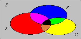
In the simple probability experiment, points are generated according to the uniform distribution on a rectangle. Move and resize the events \( A \) and \( B \) and note how the probabilities of the various events change. Create each of the following configurations. In each case, run the experiment 1000 times and compare the relative frequencies of the events to the probabilities of the events.

1. \( A \) and \( B \) in general position
2. \( A \) and \( B \) disjoint
3. \( A \subseteq B \)
4. \( B \subseteq A \)

Genetics

Please refer to the discussion of genetics in the section on random experiments if you need to review some of the definitions in this subsection.

Recall first that the ABO blood type in humans is determined by three alleles: \(a\), \(b\), and \(o\). Furthermore, \(a\) and \(b\) are co-dominant and \(o\) is recessive. Suppose that the probability distribution for the set of blood genotypes in a certain population is given in the following table:

Genotype	\(aa\)	\(ab\)	\(ao\)	\(bb\)	\(bo\)	\(oo\)
Probability	0.050	0.038	0.310	0.007	0.116	0.479

A person is chosen at random from the population. Let \(A\), \(B\), \(AB\), and \(O\) be the events that the person is type \(A\), type \(B\), type \(AB\), and type \(O\) respectively. Let \(H\) be the event that the person is homozygous and \(D\) the event that the person has an \(o\) allele. Find the probability of the following events:

1. \(A\)
2. \(B\)
3. \(AB\)
4. \(O\)
5. \(H\)
6. \(D\)
7. \(H \cup D\)
8. \(D^c\)

Answer

1. 0.360
2. 0.123
3. 0.038
4. 0.479
5. 0.536
6. 0.905
7. 0.962
8. 0.095

Suppose next that pod color in certain type of pea plant is determined by a gene with two alleles: \(g\) for green and \(y\) for yellow, and that \(g\) is dominant.

Let \(G\) be the event that a child plant has green pods. Find \(\P(G)\) in each of the following cases:

1. At least one parent is type \(gg\).
2. Both parents are type \(yy\).
3. Both parents are type \(gy\).
4. One parent is type \(yy\) and the other is type \(gy\).

Answer

1. \(1\)
2. \(0\)
3. \(\frac{3}{4}\)
4. \(\frac{1}{2}\)

Next consider a sex-linked hereditary disorder in humans (such as colorblindness or hemophilia). Let \(h\) denote the healthy allele and \(d\) the defective allele for the gene linked to the disorder. Recall that \(d\) is recessive for women.

Let \(B\) be the event that a son has the disorder, \(C\) the event that a daughter is a healthy carrier, and \(D\) the event that a daughter has the disease. Find \(\P(B)\), \(\P(C)\) and \(\P(D)\) in each of the following cases:

1. The mother and father are normal.
2. The mother is a healthy carrier and the father is normal.
3. The mother is normal and the father has the disorder.
4. The mother is a healthy carrier and the father has the disorder.
5. The mother has the disorder and the father is normal.
6. The mother and father both have the disorder.

Answer

1. \(0\), \(0\), \(0\)
2. \(1/2\), 0, \(1/2\)
3. \(0\), \(1/2\), \(0\)
4. \(1/2\), \(1/2\), \(1/2\)
5. \(1\), \(1/2\), \(0\)
6. \(1\), \(0\), \(1\)

From this exercise, note that transmission of the disorder to a daughter can only occur if the mother is at least a carrier and the father has the disorder. In ordinary large populations, this is a unusual intersection of events, and thus sex-linked hereditary disorders are typically much less common in women than in men. In brief, women are protected by the extra X chromosome.

Radioactive Emissions

Suppose that \(T\) denotes the time between emissions (in milliseconds) for a certain type of radioactive material, and that \(T\) has the following probability distribution, defined for measurable \(A \subseteq [0, \infty)\) by \[\P(T \in A) = \int_A e^{-t} \, dt\]

1. Show that this really does define a probability distribution.
2. Find \(\P(T \gt 3)\).
3. Find \(\P(2 \lt T \lt 4)\).

Answer

1. Note that \( \int_0^\infty e^{-t} \, dt = 1 \)
2. \(e^{-3}\)
3. \(e^{-2} - e^{-4}\)

Suppose that \(N\) denotes the number of emissions in a one millisecond interval for a certain type of radioactive material, and that \(N\) has the following probability distribution: \[\P(N \in A) = \sum_{n \in A} \frac{e^{-1}}{n!}, \quad A \subseteq \N\]

1. Show that this really does define a probability distribution.
2. Find \(\P(N \ge 3)\).
3. Find \(\P(2 \le N \le 4)\).

Answer

1. Note that \( \sum_{n=0}^\infty \frac{e^{-1}}{n!} = 1 \)
2. \(1 - \frac{5}{2} e^{-1}\)
3. \(\frac{17}{24} e^{-1}\)

The probability distribution that governs the time between emissions is a special case of the exponential distribution, while the probability distribution that governs the number of emissions is a special case of the Poisson distribution, named for Simeon Poisson. The exponential distribution and the Poisson distribution are studied in more detail in the chapter on the Poisson process.

Matching

Suppose that at an absented-minded secretary prepares 4 letters and matching envelopes to send to 4 different persons, but then stuffs the letters into the envelopes randomly. Find the probability of the event \(A\) that at least one letter is in the proper envelope.

Solution

Note first that the set of outcomes \( S \) can be taken to be the set of permutations of \(\{1, 2, 3, 4\}\). For \(\bs{x} \in S\), \(x_i\) is the number of the envelope containing the \(i\)th letter. Clearly \(S\) should be given the uniform probability distribution. Next note that \(A = A_1 \cup A_2 \cup A_3 \cup A_4\) where \(A_i\) is the event that the \(i\)th letter is inserted into the \(i\)th envelope. Using the inclusion-exclusion rule gives \(\P(A) = \frac{5}{8}\).

This exercise is an example of the matching problem, originally formulated and studied by Pierre Remond Montmort. A complete analysis of the matching problem is given in the chapter on Finite Sampling Models.

In the simulation of the matching experiment select \(n = 4\). Run the experiment 1000 times and compute the relative frequency of the event that at least one match occurs.

Data Analysis Exercises

For the M&M data set, let \(R\) denote the event that a bag has at least 10 red candies, \(T\) the event that a bag has at least 57 candies total, and \(W\) the event that a bag weighs at least 50 grams. Find the empirical probability the following events:

1. \(R\)
2. \(T\)
3. \(W\)
4. \(R \cap T\)
5. \(T \setminus W\)

Answer

1. \(\frac{13}{30}\)
2. \(\frac{19}{30}\)
3. \(\frac{9}{30}\)
4. \(\frac{9}{30}\)
5. \(\frac{11}{30}\)

For the cicada data, let \(W\) denote the event that a cicada weighs at least 0.20 grams, \(F\) the event that a cicada is female, and \(T\) the event that a cicada is type tredecula. Find the empirical probability of each of the following:

1. \(W\)
2. \(F\)
3. \(T\)
4. \(W \cap F\)
5. \(F \cup T \cup W\)

Answer

1. \(\frac{37}{104}\)
2. \(\frac{59}{104}\)
3. \(\frac{44}{104}\)
4. \(\frac{34}{104}\)
5. \(\frac{85}{104}\)