2.2: Events and Random Variables

Last updated
Save as PDF

Page ID: 10130

$ \newcommand{\vecs}[1]{\overset { \scriptstyle \rightharpoonup} {\mathbf{#1}} } $ $ \newcommand{\vecd}[1]{\overset{-\!-\!\rightharpoonup}{\vphantom{a}\smash {#1}}} $$\newcommand{\id}{\mathrm{id}}$ $ \newcommand{\Span}{\mathrm{span}}$ $ \newcommand{\kernel}{\mathrm{null}\,}$ $ \newcommand{\range}{\mathrm{range}\,}$ $ \newcommand{\RealPart}{\mathrm{Re}}$ $ \newcommand{\ImaginaryPart}{\mathrm{Im}}$ $ \newcommand{\Argument}{\mathrm{Arg}}$ $ \newcommand{\norm}[1]{\| #1 \|}$ $ \newcommand{\inner}[2]{\langle #1, #2 \rangle}$ $ \newcommand{\Span}{\mathrm{span}}$ $\newcommand{\id}{\mathrm{id}}$ $ \newcommand{\Span}{\mathrm{span}}$ $ \newcommand{\kernel}{\mathrm{null}\,}$ $ \newcommand{\range}{\mathrm{range}\,}$ $ \newcommand{\RealPart}{\mathrm{Re}}$ $ \newcommand{\ImaginaryPart}{\mathrm{Im}}$ $ \newcommand{\Argument}{\mathrm{Arg}}$ $ \newcommand{\norm}[1]{\| #1 \|}$ $ \newcommand{\inner}[2]{\langle #1, #2 \rangle}$ $ \newcommand{\Span}{\mathrm{span}}$$\newcommand{\AA}{\unicode[.8,0]{x212B}}$

$\newcommand{\R}{\mathbb{R}}$ $\newcommand{\N}{\mathbb{N}}$ $\newcommand{\bs}{\boldsymbol}$

The purpose of this section is to study two basic types of objects that form part of the model of a random experiment. If you are a new student of probability, just ignore the measure-theoretic terminology and skip the technical details.

Sample Spaces

The Set of Outcomes

Recall that in a random experiment, the outcome cannot be predicted with certainty, before the experiment is run. On the other hand:

We assume that we can identify a fixed set $ S $ that includes all possible outcomes of a random experiment. This set plays the role of the universal set when modeling the experiment.

For simple experiments, $ S $ may be precisely the set of possible outcomes. More often, for complex experiments, $ S $ is a mathematically convenient set that includes the possible outcomes and perhaps other elements as well. For example, if the experiment is to throw a standard die and record the score that occurs, we would let $S = \{1, 2, 3, 4, 5, 6\}$, the set of possible outcomes. On the other hand, if the experiment is to capture a cicada and measure its body weight (in milligrams), we might conveniently take $S = [0, \infty)$, even though most elements of this set are impossible (we hope!). The problem is that we may not know exactly the outcomes that are possible. Can a light bulb burn without failure for one thousand hours? For one thousand days? for one thousand years?

Often the outcome of a random experiment consists of one or more real measurements, and thus, the $ S $ consists of all possible measurement sequences, a subset of $\R^n$ for some $n \in \N_+$. More generally, suppose that we have $n$ experiments and that $ S_i $ is the set of outcomes for experiment $ i \in \{1, 2, \ldots, n\} $. Then the Cartesian product $S_1 \times S_2 \times \cdots \times S_n$ is the natural set of outcomes for the compound experiment that consists of performing the $n$ experiments in sequence. In particular, if we have a basic experiment with $S$ as the set of outcomes, then $S^n$ is the natural set of outcomes for the compound experiment that consists of $n$ replications of the basic experiment. Similarly, if we have an infinite sequence of experiments and $ S_i $ is the set of outcomes for experiment $ i \in \N_+ $, then then $S_1 \times S_2 \times \cdots$ is the natural set of outcomes for the compound experiment that consists of performing the given experiments in sequence. In particular, the set of outcomes for the compound experiment that consists of indefinite replications of a basic experiment is $S^\infty = S \times S \times \cdots $. This is an essential special case, because (classical) probability theory is based on the idea of replicating a given experiment.

Events

Consider again a random experiment with $ S $ as the set of outcomes. Certain subsets of $ S $ are referred to as events. Suppose that $ A \subseteq S $ is a given event, and that the experiment is run, resulting in outcome $ s \in S $.

If $ s \in A $ then we say that $ A $ occurs.
If $ s \notin A $ then we say that $ A $ does not occur.

Intuitively, you should think of an event as a meaningful statement about the experiment: every such statement translates into an event, namely the set of outcomes for which the statement is true. In particular, $S$ itself is an event; by definition it always occurs. At the other extreme, the empty set $\emptyset$ is also an event; by definition it never occurs.

For a note on terminology, recall that a mathematical space consists of a set together with other mathematical structures defined on the set. An example you may be familiar with is a vector space, which consists of a set (the vectors) together with the operations of addition and scalar multiplication. In probability theory, many authors use the term sample space for the set of outcomes of a random experiment, but here is the more careful definition:

The sample space of an experiment is $ (S, \mathscr S) $ where $ S $ is the set of outcomes and $ \mathscr S $ is the collection of events.

Details

Sometimes not every subset of $S$ can be allowed as an event, but the collection of events $ \mathscr S $ is required to be a $ \sigma $-algebra, so that the sample space $ (S, \mathscr S) $ is a measurable space. The axioms of a $\sigma$-algebra ensure that new sets that are constructed in a reasonable way from given events, using the set operations, are themselves valid events. Most of the sample spaces that occur in elementary probability fall into two general categories.

Discrete: $ S $ is countable and $ \mathscr S = \mathscr P(S) $ is the collection of all subsets of $ S $. In this case, the sample space $(S, \mathscr S)$ is discrete.
Euclidean: $S$ is a measurable subset of $\R^n$ for some $n \in \N_+$ and $\mathscr S$ is the collection of measurable subsets of $S$.

In (b), the mearuable subsets of $\R^n$ include all of the sets encountered in calculus and in standard applications of probability theory, and many more besides. Nonetheless, for technical reasons, certain very weird subsets must be excluded. Typically $ S $ is a set defined by a finite number of inequalities involving elementary functions.

The Algebra of Events

The standard algebra of sets leads to a grammar for discussing random experiments and allows us to construct new events from given events. In the following results, suppose that $ S $ is the set of outcomes of a random experiment, and that $A$ and $B$ are events.

$A \subseteq B$ if and only if the occurrence of $A$ implies the occurrence of $B$.

Proof

Recall that $ \subseteq $ is the subset relation. So by definition, $ A \subseteq B $ means that $ s \in A $ implies $ s \in B $.

$A \cup B$ is the event that occurs if and only if $A$ occurs or $B$ occurs.

Proof

Recall that $ A \cup B $ is the union of $ A $ and $ B $. So by defintion, $ s \in A \cup B $ if and only if $ s \in A $ or $ s \in B $.

$A \cap B$ is the event that occurs if and only if $A$ occurs and $B$ occurs.

Proof

Recall that $ A \cap B $ is the intersection of $ A $ and $ B $. So by definiton, $ s \in A \cap B $ if and only if $ s \in A $ and $ s \in B $.

$A$ and $B$ are disjoint if and only if they are mutually exclusive; they cannot both occur on the same run of the experiment.

Proof

By definition, $ A $ and $ B $ disjoint means that $ A \cap B = \emptyset $.

$A^c$ is the event that occurs if and only if $A$ does not occur.

Proof

Recall that $ A^c $ is the complement of $ A $, so $ s \in A^c $ if and only if $ s \notin A $.

$A \setminus B$ is the event that occurs if and only if $A$ occurs and $B$ does not occur.

Proof

Recall that $ A \setminus B = A \cap B^c $. Hence $ s \in A \setminus B $ if and only if $ s \in A $ and $ s \notin B $.

$(A \cap B^c) \cup (B \cap A^c)$ is the event that occurs if and only if one but not both of the given events occurs.

Proof

The events in the union are disjoint. So for $ s $ is in the given event if and only if either $ s \in A $ and $ s \notin B $, or $ s \in B $ and $ s \notin A $.

Recall that the event in (10) is the symmetric difference of $A$ and $B$, and is sometimes denoted $A \Delta B$. This event corresponds to exclusive or, as opposed to the ordinary union $ A \cup B $ which corresponds to inclusive or.

$(A \cap B) \cup (A^c \cap B^c)$ is the event that occurs if and only if both or neither of the given events occurs.

Proof

The events in the union are disjoint. Thus $ s $ is in the given event if and only if either $ s \in A $ and $ s \in B $, or $ s \notin A $ and $ s \notin B $.

In the Venn diagram app, observe the diagram of each of the 16 events that can be constructed from $A$ and $B$.

Suppose now that $\mathscr{A} = \{A_i: i \in I\}$ is a collection of events for the random experiment, where $I$ is a countable index set.

$ \bigcup \mathscr{A} = \bigcup_{i \in I} A_i $ is the event that occurs if and only if at least one event in the collection occurs.

Proof

Note that $ s \in \bigcup_{i \in I} A_i $ if and only if $ s \in A_i $ for some $ i \in I $.

$ \bigcap \mathscr{A} = \bigcap_{i \in I} A_i $ is the event that occurs if and only if every event in the collection occurs:

Proof

Note that $ s \in \bigcap_{i \in I} A_i $ if and only if $ s \in A_i $ for every $ i \in I $.

$\mathscr{A}$ is a pairwise disjoint collection if and only if the events are mutually exclusive; at most one of the events could occur on a given run of the experiment.

Proof

By definition, $ A_i \cap A_j = \emptyset $ for distinct $ i, \, j \in I $.

Suppose now that $(A_1, A_2, \ldots$) is an infinite sequence of events.

$\bigcap_{n=1}^\infty \bigcup_{i=n}^\infty A_i$ is the event that occurs if and only if infinitely many of the given events occur. This event is sometimes called the limit superior of $(A_1, A_2, \ldots)$.

Proof

Note that $ s $ is in the given event if and only if for every $ n \in \N_+ $ there exists $ i \in \N_+ $ with $ i \ge n $ such that $ s \in A_i $. In turn this means that $ s \in A_i $ for infinitely many $ i \in I $.

$\bigcup_{n=1}^\infty \bigcap_{i=n}^\infty A_i$ is the event that occurs if and only if all but finitely many of the given events occur. This event is sometimes called the limit inferior of $(A_1, A_2, \ldots)$.

Proof

Note that $ s $ is in the given event if and only if there exists $ n \in \N_+ $ such that $ s \in A_i $ for every $ i \in \N_+ $ with $ i \ge n $. In turn, this means that $ s \in A_i $ for all but finitely many $ i \in I $.

Limit superiors and inferiors are discussed in more detail in the section on convergence.

Random Variables

Intuitively, a random variable is a measurement of interest in the context of the experiment. Simple examples include the number of heads when a coin is tossed several times, the sum of the scores when a pair of dice are thrown, the lifetime of a device subject to random stress, the weight of a person chosen from a population. Many more examples are given below in the exercises below. Mathematically, a random variable is a function defined on the set of outcomes.

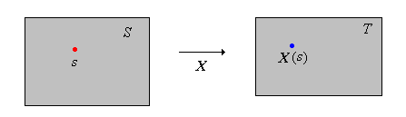
A function $ X $ from $ S $ into a set $ T $ is a random variable for the experiment with values in $ T $.

Details

The set $ T $ will also come with a $ \sigma $-algebra $ \mathscr T $ of admissible subsets, so that $(T, \mathscr T)$ is a measurable space, just like $ (S, \mathscr S) $. The function $ X $ is required to be measurable, an assumption which ensures that meaningful statements involving $ X $ define events. In the discussion below, all subsets of $ T $ are assumed to be in $ \mathscr T $.

Probability has its own notation, very different from other branches of mathematics. As a case in point, random variables, even though they are functions, are usually denoted by capital letters near the end of the alphabet. The use of a letter near the end of the alphabet is intended to emphasize the idea that the object is a variable in the context of the experiment. The use of a capital letter is intended to emphasize the fact that it is not an ordinary algebraic variable to which we can assign a specific value, but rather a random variable whose value is indeterminate until we run the experiment. Specifically, when we run the experiment an outcome $s \in S$ occurs, and random variable $X$ takes the value $X(s) \in T$.

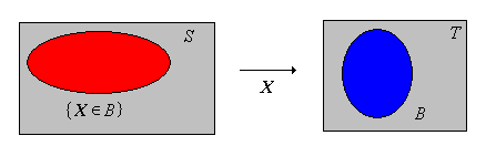
If $ B \subseteq T $, we use the notation $ \{X \in B\} $ for the inverse image $ \{s \in S: X(s) \in B\} $, rather than $ X^{-1}(B) $. Again, the notation is more natural since we think of $ X $ as a variable in the experiment. Think of $ \{X \in B\} $ as a statement about $ X $, which then translates into the event $ \{s \in S: X(s) \in B\} $

An event defined by a random variable — Figure $\PageIndex{2}$: The event $ \{X \in B\} $ corresponding to $ B \subseteq T $

Again, every statement about a random variable $ X $ with values in $ T $ translates into an inverse image of the form $ \{X \in B\} $ for some $ B \in \mathscr T $. So, for example, if $ x \in T $ then $\{X = x\} = \{X \in \{x\}\} = \left\{s \in S: X(s) = x\right\}$. If $X$ is a real-valued random variable and $ a, \, b \in \R $ with $ a \lt b $ then $\{ a \leq X \leq b\} = \left\{ X \in [a, b]\right\} = \{s \in S: a \leq X(s) \leq b\}$.

Suppose that $X$ is a random variable taking values in $T$, and that $A, \, B \subseteq T$. Then

$\{X \in A \cup B\} = \{X \in A\} \cup \{X \in B\}$
$\{X \in A \cap B\} = \{X \in A\} \cap \{X \in B\}$
$\{X \in A \setminus B\} = \{X \in A\} \setminus \{X \in B\}$
$A \subseteq B \implies \{X \in A\} \subseteq \{X \in B\}$
If $A$ and $B$ are disjoint, then so are $\{X \in A\}$ and $\{X \in B\}$.

Proof

This is a restatement of the fact that inverse images of a function preserve the set operations; only the notation changes (and is simpler).

$s \in \{X \in A \cup B\}$ if and only if $X(s) \in A \cup B$ if and only if $X(s) \in A$ or $X(s) \in B$ if and only if $s \in \{X \in A\}$ or $s \in \{X \in B\}$ if and only if $s \in \{X \in A\} \cup \{X \in B\}$.
The proof is exactly the same as (a), with and replacing or.
The proof is also exactly the same as (a), with but not replacing or.
If $s \in \{X \in A\}$ then $X(s) \in A$ so $X(s) \in B$ and hence $s \in \{X \in B\}$.
This follows from part (b).

As with a general function, the result in part (a) holds for the union of a countable collection of subsets, and the result in part (b) holds for the intersection of a countable collection of subsets. No new ideas are involved; only the notation is more complicated.

Often, a random variable takes values in a subset $T$ of $\R^k$ for some $k \in \N_+$. We might express such a random variable as $\bs{X} = (X_1, X_2, \ldots, X_k)$ where $X_i$ is a real-valued random variable for each $i \in \{1, 2, \ldots, k\}$. In this case, we usually refer to $\bs{X}$ as a random vector, to emphasize its higher-dimensional character. A random variable can have an even more complicated structure. For example, if the experiment is to select $n$ objects from a population and record various real measurements for each object, then the outcome of the experiment is a vector of vectors: $\bs{X} = (X_1, X_2, \ldots, X_n)$ where $X_i$ is the vector of measurements for the $i$th object. There are other possibilities; a random variable could be an infinite sequence, or could be set-valued. Specific examples are given in the computational exercises below. However, the important point is simply that a random variable is a function defined on the set of outcomes $S$.

The outcome of the experiment itself can be thought of as a random variable. Specifically, let $T = S$ and let $X$ denote the identify function on $S$ so that $X(s) = s$ for $s \in S$. Then trivially $X$ is a random variable, and the events that can be defined in terms of $X$ are simply the original events of the experiment. That is, if $ A $ is an event then $ \{X \in A\} = A $. Conversely, every random variable effectively defines a new random experiment.

In the general setting above, a random variable $X$ defines a new random experiment with $ T $ as the new set of outcomes and subsets of $ T $ as the new collection of events.

Details

Technically, the $ \sigma $-algebra $ \mathscr T $ would be the new collection of events.

In fact, often a random experiment is modeled by specifying the random variables of interest, in the language of the experiment. Then, a mathematical definition of the random variables specifies the sample space. A function (or transformation) of a random variable defines a new random variable.

Suppose that $ X $ is a random variable for the experiment with values in $T$ and that $ g $ is a function from $ T $ into another set $ U $. Then $ Y = g(X) $ is a random variable with values in $ U $.

Details

Technically, $ T $ and $ U $ both come with $\sigma$-algebras of admissible subsets $ \mathscr T $ and $ \mathscr U $, respectively. The function $ g $, just like the function $ X $, is required to be measurable. This assumption ensures that $Y = g(X)$ is a measurable function from $S$ into $U$, and hence is a valid random variable.

Note that, as functions, $ g(X) = g \circ X $, the composition of $ g $ with $ X $. But again, thinking of $ X $ and $ Y $ as variables in the context of the experiment, the notation $ Y = g(X) $ is much more natural.

Indicator Variables

For an event $A$, the indicator function of $A$ is called the indicator variable of $A$.

The value of this random variables tells us whether or not $A$ has occurred: \[ \bs{1}_A = \begin{cases} 1, & A \text{ occurs} \\ 0, & A \text{ does not occur} \end{cases} \] That is, as a function on $ S $, \[ \bs{1}_A(s) = \begin{cases} 1, & s \in A \\ 0, & s \notin A \end{cases} \]

If $X$ is a random variable that takes values 0 and 1, then $X$ is the indicator variable of the event $\{X = 1\}$.

Proof

Note that for $ s \in S $, $ X(s) = 1$ if $ s \in \{X = 1\} $ and $ X(s) = 0 $ otherwise.

Recall also that the set algebra of events translates into the arithmetic algebra of indicator variables.

Suppose that $A$ and $B$ are events.

$\bs{1}_{A \cap B} = \bs{1}_A \bs{1}_B = \min\left\{\bs{1}_A, \bs{1}_B\right\}$
$\bs{1}_{A \cup B} = 1 - \left(1 - \bs{1}_A\right)\left(1 - \bs{1}_B\right) = \max\left\{\bs{1}_A, \bs{1}_B\right\}$
$\bs{1}_{B \setminus A} = \bs{1}_B \left(1 - \bs{1}_A\right)$
$\bs{1}_{A^c} = 1 - \bs{1}_A$
$A \subseteq B$ if and only if $\bs{1}_A \leq \bs{1}_B$

The results in part (a) extends to arbitrary intersections and the results in part (b) extends to arbitrary unions. If the event $ A $ has a complicated description, sometimes we use $ \bs 1 (A) $ for the indicator variable rather that $ \bs 1_A $.

Examples and Applications

Recall that probability theory is often illustrated using simple devices from games of chance: coins, dice, cards, spinners, urns with balls, and so forth. Examples based on such devices are pedagogically valuable because of their simplicity and conceptual clarity. On the other hand, remember that probability is not only about gambling and games of chance. Rather, try to see problems involving coins, dice, etc. as metaphors for more complex and realistic problems.

Coins and Dice

The basic coin experiment consists of tossing a coin $n$ times and recording the sequence of scores $(X_1, X_2, \ldots, X_n)$ (where 1 denotes heads and 0 denotes tails). This experiment is a generic example of $n$ Bernoulli trials, named for Jacob Bernoulli.

Consider the coin experiment with $n = 4$, and Let $Y$ denote the number of heads.

Give the set of outcomes $S$ in list form.
Give the event $\{Y = k\}$ in list form for each $k \in \{0, 1, 2, 3, 4\}$.

Answer

To simplify the notation, we represent outcomes a bit strings rather than ordered sequences.

$S = \{1111, 1110, 1101, 1011, 0111, 1100, 1010, 1001, 0110, 0101, 0011, 1000, 0100, 0010, 0001, 0000\}$
\begin{align} \{Y = 0\} & = \{0000\} \\ \{Y = 1\} & = \{1000, 0100, 0010, 0001\} \\ \{Y = 2\} & = \{1100, 1010, 1001, 0110, 0101, 0011\} \\ \{Y = 3\} & = \{1110, 1101, 1011, 0111\} \\ \{Y = 4\} & = \{1111\} \end{align}

In the simulation of the coin experiment, set $n = 4$. Run the experiment 100 times and count the number of times that the event $\{Y = 2\}$ occurs.

Now consider the general coin experiment with the coin tossed $n$ times, and let $Y$ denote the number of heads.

Give the set of outcomes $S$ in Cartesian product form, and give the cardinality of $S$.
Express $Y$ as a function on $S$.
Find $\#\{Y = k\}$ (as a subset of $S$) for $k \in \{0, 1, \ldots, n\}$

Answer

$S = \{0, 1\}^n$ and $\#(S) = 2^n$.
$Y(x_1, x_2, \ldots, x_n) = x_1 + x_2 + \cdots + x_n$. The set of possible values is $\{0, 1, \ldots, n\}$
$\#\{Y = k\} = \binom{n}{k}$

The basic dice experiment consists of throwing $n$ distinct $k$-sided dice (with faces numbered from 1 to $k$) and recording the sequence of scores $(X_1, X_2, \ldots, X_n)$. This experiment is a generic example of $n$ multinomial trials. The special case $k = 6$ corresponds to standard dice.

Consider the dice experiment with $n = 2$ standard dice. Let $S$ denote the set of outcomes, $A$ the event that the first die score is 1, and $B$ the event that the sum of the scores is 7. Give each of the following events in the form indicated:

$S$ in Cartesian product form
$A$ in list form
$B$ in list form
$A \cup B$ in list form
$A \cap B$ in list form
$A^c \cap B^c$ in predicate form

Answer

$S = \{1, 2, 3, 4, 5, 6\}^2$
$A = \{(1,1), (1,2), (1,3), (1,4), (1,5), (1,6)\}$
$B = \{(1,6), (2,5), (3,4), (4,3), (5,2), (6,1)\}$
$A \cup B = \{(1,1), (1,2), (1,3), (1,4), (1,5), (1,6), (2,5), (3,4), (4,3), (5,2), (6,1)\}$
$A \cap B = \{(1,6)\}$
$A^c \cap B^c = \{(x, y) \in S: x + y \ne 7 \text{ and } x \ne 1\}$

In the simulation of the dice experiment, set $n = 2$. Run the experiment 100 times and count the number of times each event in the previous exercise occurs.

Consider the dice experiment with $n = 2$ standard dice, and let $ S $ denote the set of outcomes, $Y$ the sum of the scores, $U$ the minimum score, and $V$ the maximum score.

Express $Y$ as a function on $ S $ and give the set of possible values in list form.
Express $U$ as a function on $ S $ and give the set of possible values in list form.
Express $V$ as a function on the $ S $ and give the set of possible values in list form.
Give the set of possible values of $(U, V)$ in predicate from

Answer

Note that $ S = \{1, 2, 3, 4, 5, 6\}^2 $. The following functions are defined on $ S $.

$Y(x_1, x_2) = x_1 + x_2$. The set of values is $\{2, 3, \ldots, 12\}$
$U(x_1, x_2) = \min\{x_1, x_2\}$. The set of values is $\{1, 2, \ldots, 6\}$
$V(x_1, x_2) = \max\{x_1, x_2\}$. The set of values is $\{1, 2, \ldots, 6\}$
$\left\{(u, v) \in \{1, 2, 3, 4, 5, 6\}^2: u \le v\right\}$

Consider again the dice experiment with $n = 2$ standard dice, and let $ S $ denote the set of outcomes, $Y$ the sum of the scores, $U$ the minimum score, and $V$ the maximum score. Give each of the following as subsets of $ S $, in list form.

$\{X_1 \lt 3, X_2 \gt 4\}$
$\{Y = 7\}$
$\{U = 2\}$
$\{V = 4\}$
$\{U = V\}$

Answer

$\{(1,5), (2,5), (1,6), (2,6)\}$
$\{(1,6), (2,5), (3,4), (4,3), (5,2), (6,1)\}$
$\{(2,2), (2,3), (3,2), (2,4), (4,2), (2,5), (5,2), (2,6), (6,2)\}$
$\{(4,1), (1,4), (2,4), (4,2), (4,3), (3,4), (4,4)\}$
$\{(1,1), (2,2), (3,3), (4,4), (5,5), (6,6)\}$

In the dice experiment, set $n = 2$. Run the experiment 100 times. Count the number of times each event in the previous exercise occurred.

In the general dice experiment with $n$ distinct $k$-sided dice, let $Y$ denote the sum of the scores, $U$ the minimum score, and $V$ the maximum score.

Give the set of outcomes $ S $ and find $ \#(S) $.
Express $Y$ as a function on $ S $, and give the set of possible values in list form.
Express $U$ as a function on $ S $, and give the set of possible values in list form.
Express $V$ as a function on $ S $, and give the set of possible values in list form.
Give the set of possible values of $(U, V)$ in predicate from.

Answer

$S = \{1, 2, \ldots, k\}^n$ and $\#(S) = k^n$
$Y(x_1, x_2, \ldots, x_n) = x_1 + x_2 + \cdots + x_n$. The set of possible values is $\{n, n + 1, \ldots, n k\}$
$U(x_1, x_2, \ldots, x_n) = \min\{x_1, x_2, \ldots, x_n\}$. The set of possible values is $\{1, 2, \ldots, k\}$.
$V(x_1, x_2, \ldots, x_n) = \max\{x_1, x_2 \ldots, x_n\}$. The set of possible values is $\{1, 2, \ldots, k\}$
$\left\{(u, v) \in \{1, 2, \ldots, k\}^2: u \le v\right\}$

The set of outcomes of a random experiment depends of course on what information is recorded. The following exercise is an illustration.

An experiment consists of throwing a pair of standard dice repeatedly until the sum of the two scores is either 5 or 7. Let $A$ denote the event that the sum is 5 rather than 7 on the final throw. Experiments of this type arise in the casino game craps.

Suppose that the pair of scores on each throw is recorded. Define the set of outcomes of the experiment and describe $A$ as a subset of this set.
Suppose that the pair of scores on the final throw is recorded. Define the set of outcomes of the experiment and describe $A$ as a subset of this set.

Answer

Let $D_5 = \{(1,4), (2,3), (3,2), (4,1)\}$, $D_7 = \{(1,6), (2,5), (3,4), (4,3), (5,2), (6,1)\}$, $D = D_5 \cup D_7 $, and $ C = D^c $

$S = D \cup (C \times D) \cup (C^2 \times D) \cup \cdots$, $A = D_5 \cup (C \times D_5) \cup (C^2 \times D_5) \cup \cdots$
$S = D$, $A = D_5$

Suppose that 3 standard dice are rolled and the sequence of scores $(X_1, X_2, X_3)$ is recorded. A person pays $1 to play. If some of the dice come up 6, then the player receives her $1 back, plus $1 for each 6. Otherwise she loses her $1. Let $W$ denote the person's net winnings. This is the game of chuck-a-luck and is treated in more detail in the chapter on Games of Chance.

Give the set of outcomes $S$ in Cartesian product form.
Express $W$ as a function on $S$ and give the set of possible values in list form.

Answer

$S = \{1, 2, 3, 4, 5, 6\}^3$
$W(x_1, x_2, x_3) = \bs{1}\left(x_1 = 6\right) + \bs{1}\left(x_2 = 6\right) + \bs{1}\left(x_3 = 6\right) - \bs{1}\left(x_1 \ne 6, x_2 \ne 6, x_3 \ne 6\right)$. The set of possible values is $\{-1, 1, 2, 3\}$

Play the chuck-a-luck experiment a few times and see how you do.

In the die-coin experiment, a standard die is rolled and then a coin is tossed the number of times shown on the die. The sequence of coin scores $\bs{X}$ is recorded (0 for tails, 1 for heads). Let $N$ denote the die score and $Y$ the number of heads.

Give the set of outcomes $S$ in terms of Cartesian powers and find $\#(S)$.
Express $N$ as a function on $S$ and give the set of possible values in list form.
Express $Y$ as a function on $S$ and give the set of possible values in list form.
Give the event $A$ that all tosses result in heads in list form.

Answer

$S = \bigcup_{n=1}^6 \{0, 1\}^n$, $\#(S) = 126$
$N(x_1, x_2, \ldots, x_n) = n$ for $(x_1, x_2, \ldots, x_n) \in S$. The set of values is $\{1, 2, 3, 4, 5, 6\}$.
$Y(x_1, x_2, \ldots, x_n) = \sum_{i=1}^n x_i$ for $(x_1, x_2, \ldots, x_n) \in S$. The set of possible values is $\{0, 1, 2, 3, 4, 5, 6\}$.
$A = \{1, 11, 111, 1111, 11111, 111111\}$

Run the simulation of the die-coin experiment 10 times. For each run, give the values of the random variables $\bs{X}$, $N$, and $Y$ of the previous exercise. Count the number of times the event $A$ occurs.

In the coin-die experiment, we have a coin and two distinct dice, say one red and one green. First the coin is tossed, and then if the result is heads the red die is thrown, while if the result is tails the green die is thrown. The coin score $X$ and the score of the chosen die $Y$ are recorded. Suppose now that the red die is a standard 6-sided die, and the green die a 4-sided die.

Give the set of outcomes $S$ in list form.
Express $X$ as a function on $ S $.
Express $Y$ as a function on $ S $.
Give the event $\{Y \ge 3\}$ as a subset of $ S $ in list form.

Answer

$\{(0,1), (0,2), (0,3), (0,4), (1,1), (1,2), (1,3), (1,4), (1,5), (1,6)\}$
$X(i, j) = i$ for $(i, j) \in S$
$Y(i, j) = j$ for $(i, j) \in S$
$\{(0,3), (0,4), (1,3), (1,4), (1,5), (1,6)\}$

Run the coin-die experiment 100 times, with various types of dice.

Sampling Models

Recall that many random experiments can be thought of as sampling experiments. For the general finite sampling model, we start with a population $D$ with $m$ (distinct) objects. We select a sample of $n$ objects from the population. If the sampling is done in a random way, then we have a random experiment with the sample as the basic outcome. Thus, the set of outcomes of the experiment is literally the set of samples; this is the historical origin of the term sample space. There are four common types of sampling from a finite population, based on the criteria of order and replacement. Recall the following facts from the section on combinatorial structures:

Samples of size $ n $ chosen from a population with $ m $ elements.

If the sampling is with replacement and with regard to order, then the set of samples is the Cartesian power $D^n$. The number of samples is $m^n$.
If the sampling is without replacement and with regard to order, then the set of samples is the set of all permutations of size $n$ from $D$. The number of samples is $m^{(n)} = m (m - 1) \cdots [m - (n - 1)]$.
If the sampling is without replacement and without regard to order, then the set of samples is the set of all combinations (or subsets) of size $n$ from $D$. The number of samples is $\binom{m}{n}$.
If the sampling is with replacement and without regard to order, then the set of samples is the set of all multisets of size $n$ from $D$. The number of samples is $\binom{m + n - 1}{n}$.

If we sample with replacement, the sample size $n$ can be any positive integer. If we sample without replacement, the sample size cannot exceed the population size, so we must have $n \in \{1, 2, \ldots, m\}$.

The basic coin and dice experiments are examples of sampling with replacement. If we toss a coin $n$ times and record the sequence of scores (where as usual, 0 denotes tails and 1 denotes heads), then we generate an ordered sample of size $n$ with replacement from the population $\{0, 1\}$. If we throw $n$ (distinct) standard dice and record the sequence of scores, then we generate an ordered sample of size $n$ with replacement from the population $\{1, 2, 3, 4, 5, 6\}$.

Suppose that the sampling is without replacement (the most common case). If we record the ordered sample $\bs{X} = (X_1, X_2, \ldots, X_n)$, then the unordered sample $\bs{W} = \{X_1, X_2, \ldots, X_n\}$ is a random variable (that is, a function of $\bs{X}$). On the other hand, if we just record the unordered sample $\bs{W}$ in the first place, then we cannot recover the ordered sample. Note also that the number of ordered samples of size $n$ is simply $n!$ times the number of unordered samples of size $n$. No such simple relationship exists when the sampling is with replacement. This will turn out to be an important point when we study probability models based on random samples, in the next section.

Consider a sample of size $n = 3$ chosen without replacement from the population $\{a, b, c, d, e\}$.

Give $T$, the set of unordered samples in list form.
Give in list form the set of all ordered samples that correspond to the unordered sample $\{b, c, e\}$.
Note that for every unordered sample, there are 6 ordered samples.
Give the cardinality of $S$, the set of ordered samples.

Answer

$T = \left\{\{a,b,c\}, \{a,b,d\}, \{a,b,e\}, \{a,c,d\}, \{a,c,e\}, \{a,d,e\}, \{b,c,d\}, \{b,c,e\}, \{b,d,e\}, \{c,d,e\}\right\}$
$\{(b,c,e), (b,e,c), (c,b,e), (c,e,b), (e,b,c), (e,c,b)\}$
60

Traditionally in probability theory, an urn containing balls is often used as a metaphor for a finite population.

Suppose that an urn contains 50 (distinct) balls. A sample of 10 balls is selected from the urn. Find the number of samples in each of the following cases:

Ordered samples with replacement
Ordered samples without replacement
Unordered samples without replacement
Unordered samples with replacement

Answer

$97\,656\,250\,000\,000\,000$
$37\,276\,043\,023\,296\,000$
$10\,272\,278\,170$
$62\,828\,356\,305$

Suppose again that we have a population $D$ with $m$ (distinct) objects, but suppose now that each object is one of two types—either type 1 or type 0. Such populations are said to be dichotomous. Here are some specific examples:

The population consists of persons, each either male or female.
The population consists of voters, each either democrat or republican.
The population consists of devices, each either good or defective.
The population consists of balls, each either red or green.

Suppose that the population $D$ has $r$ type 1 objects and hence $m - r$ type 0 objects. Of course, we must have $r \in \{0, 1, \ldots, m\}$. Now suppose that we select a sample of size $n$ without replacement from the population. Note that this model has three parameters: the population size $m$, the number of type 1 objects in the population $r$, and the sample size $n$.

Let $Y$ denote the number of type 1 objects in the sample. Then

$\#\{Y = k\} = \binom{n}{k} r^{(k)} (m - r)^{(n - k)}$ for each $k \in \{0, 1, \ldots, n\}$, if the event is considered as a subset of $S$, the set of ordered samples.
$\#\{Y = k\} = \binom{r}{k} \binom{m - r}{n - k}$ for each $k \in \{0, 1, \ldots, n\}$, if the event is considered as a subset of $T$, the set of unordered samples.
The expression in (a) is $n!$ times the expression in (b).

Proof

$\binom{n}{k}$ is the number of ways to pick the coordinates (in the ordered sample) where the type 1 objects will go, $r^{(k)}$ is the number of ways to select a permutation of $k$ type 1 objects, and $(m - r)^{(n-k)}$ is the number of ways to select a permutation of $n - k$ type 0 objects. The result follows from the multiplication principle.
$\binom{r}{k}$ is the number of ways to select a combatination of $k$ type 1 objects and $\binom{m - r}{n - k}$ is the number of ways to select a combination of $n - k$ type 0 objects. The result again follows from the multiplication principle.
This result can be shown algebraically, but a combinatorial argument is better. For every combination of size $n$ there are $n!$ permutations of those objects.

A batch of 50 components consists of 40 good components and 10 defective components. A sample of 5 components is selected, without replacement. Let $Y$ denote the number of defectives in the sample.

Let $S$ denote the set of ordered samples. Find $\#(S)$.
Let $T$ denote the set of unordered samples. Find $\#(T)$.
As a subset of $T$, find $\#\{Y = k\}$ for each $k \in \{0, 1, 2, 3, 4, 5\}$.

Answer

$254\,251\,200$
$2\,118\,760$
$\#\{Y = 0\} = 658\,008$, $\#\{Y = 1\} = 913\,900$, $\#\{Y = 2\} = 444\,600$, $\#\{Y = 3\} = 93\,600$, $\#\{Y = 4\} = 8\,400$, $\#\{Y = 5\} = 252$

Run the simulation of the ball and urn experiment 100 times for the parameter values in the last exercise: $ m = 50 $, $ r = 10 $, $ n = 5 $. Note the values of the random variable $Y$.

Cards

Recall that a standard card deck can be modeled by the Cartesian product set \[D = \{1, 2, 3, 4, 5, 6, 7, 8, 9, 10, j, q, k\} \times \{\clubsuit, \diamondsuit, \heartsuit, \spadesuit\}\] where the first coordinate encodes the denomination or kind (ace, 2–10, jack, queen, king) and where the second coordinate encodes the suit (clubs, diamonds, hearts, spades). Sometimes we represent a card as a string rather than an ordered pair (for example $q \heartsuit$ rather than $(q, \heartsuit)$ for the queen of hearts).

Most card games involve sampling without replacement from the deck $D$, which plays the role of the population. Thus, the basic card experiment consists of dealing $n$ cards from a standard deck without replacement; in this special context, the sample of cards is often referred to as a hand. Just as in the general sampling model, if we record the ordered hand $\bs{X} = (X_1, X_2, \ldots, X_n)$, then the unordered hand $\bs{W} = \{X_1, X_2, \ldots, X_n\}$ is a random variable (that is, a function of $\bs{X}$). On the other hand, if we just record the unordered hand $\bs{W}$ in the first place, then we cannot recover the ordered hand. Finally, recall that $n = 5$ is the poker experiment and $n = 13$ is the bridge experiment. The game of poker is treated in more detail in the chapter on Games of Chance.

Suppose that a single card is dealt from a standard deck. Let $Q$ denote the event that the card is a queen and $H$ the event that the card is a heart. Give each of the following events in list form:

$Q$
$H$
$Q \cup H$
$Q \cap H$
$Q \setminus H$

Answer

$Q = \{q \clubsuit, q \diamondsuit, q \heartsuit, q \spadesuit\}$
$H = \{1 \heartsuit, 2 \heartsuit, \ldots, 10 \heartsuit, j \heartsuit, q \heartsuit, k \heartsuit\}$
$Q \cup H = \{1 \heartsuit, 2 \heartsuit, \ldots, 10 \heartsuit, j \heartsuit, q \heartsuit, k \heartsuit, q \clubsuit, q \diamondsuit, q \spadesuit\}$
$Q \cap H = \{q \heartsuit\}$
$Q \setminus H = \{q \clubsuit, q \diamondsuit, q \spadesuit\}$

In the card experiment, set $n = 1$. Run the experiment 100 times and count the number of times each event in the previous exercise occurs.

Suppose that two cards are dealt from a standard deck and the sequence of cards recorded. Let $ S $ denote the set of outcomes, and let $Q_i$ denote the event that the $i$th card is a queen and $H_i$ the event that the $i$th card is a heart for $i \in \{1, 2\}$. Find the number of outcomes in each of the following events:

$S$
$H_1$
$H_2$
$H_1 \cap H_2$
$Q_1 \cap H_1$
$Q_1 \cap H_2$
$H_1 \cup H_2$

Answer

2652
663
663
156
51
51
1170

Consider the general card experiment in which $n$ cards are dealt from a standard deck, and the ordered hand $\bs{X}$ is recorded.

Give cardinality of $S$, the set of values of the ordered hand $ \bs{X} $.
Give the cardinality of $T$, the set of values of the unordered hand $\bs{W}$.
How many ordered hands correspond to a given unordered hand?
Explicitly compute the numbers in (a) and (b) when $n = 5$ (poker).
Explicitly compute the numbers in (a) and (b) when $n = 13$ (bridge).

Answer

$\#(S) = 52^{(n)}$
$\#(T) = \binom{52}{n}$
$n!$
$311\,875\,200$, $2\,598\,960$
$3\,954\,242\,643\,911\,239\,680\,000$, $635\,013\,559\,600$

Consider the bridge experiment of dealing 13 cards from a deck and recording the unordered hand. In the most common point counting system, an ace is worth 4 points, a king 3 points, a queen 2 points, and a jack 1 point. The other cards are worth 0 points. Let $ S $ denote the set of outcomes of the experiment and $V$ the point value of the hand.

Find the set of possible values of $V$.
Find the cardinality of the event $\{V = 0\}$ as a subset of $ S $.

Answer

$\{0, 1, \ldots, 37\}$
$\#\{V = 0\} = 2\,310\,789\,600$

In the card experiment, set $n = 13$ and run the experiment 100 times. For each run, compute the value of each of the random variable $V$ in the previous exercise.

Consider the poker experiment of dealing 5 cards from a deck. Find the cardinality of each of the events below, as a subset of the set of unordered hands.

$A$: the event that the hand is a full house (3 cards of one kind and 2 of another kind).
$B$: the event that the hand has 4 of a kind (4 cards of one kind and 1 of another kind).
$C$: the event that all cards in the hand are in the same suit (the hand is a flush or a straight flush).

Answer

$\#(A) = 3744$
$\#(B) = 624$
$\#(C) = 5148$

Run the poker experiment 1000 times. Note the number of times that the events $A$, $B$, and $C$ in the previous exercise occurred.

Consider the bridge experiment of dealing 13 cards from a standard deck. Let $ S $ denote the set of unordered hands, $Y$ the number of hearts in the hand, and $Z$ the number of queens in the hand.

Find the cardinality of the event $\{Y = y\}$ as a subset of $ S $ for each $y \in \{0, 1, \ldots, 13\}$.
Find the cardinality of the event $\{Z = z\}$ as a subset of $ S $ for each $z \in \{0, 1, 2, 3, 4\}$.

Answer

$\#(Y = y) = \binom{13}{y} \binom{39}{13 - y}$ for $y \in \{0, 1, \ldots, 13\}$
$\#(Z = z) = \binom{4}{z} \binom{48}{4 - z}$ for $z \in \{0, 1, 2, 3, 4\}$

Geometric Models

In the experiments that we have considered so far, the sample spaces have all been discrete (so that the set of outcomes is finite or countably infinite). In this subsection, we consider Euclidean sample spaces where the set of outcomes $S$ is continuous in a sense that we will make clear later. The experiments we consider are sometimes referred to as geometric models because they involve selecting a point at random from a Euclidean set.

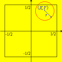
We first consider Buffon's coin experiment, which consists of tossing a coin with radius $r \le \frac{1}{2}$ randomly on a floor covered with square tiles of side length 1. The coordinates $(X, Y)$ of the center of the coin are recorded relative to axes through the center of the square in which the coin lands. Buffon's experiments are studied in more detail in the chapter on Geometric Models and are named for Compte de Buffon

Figure $\PageIndex{3}$: Buffon's coin experiment

In Buffon's coin experiment, let $ S $ denote the set of outcomes, $A$ the event that the coin does not touch the sides of the square, and let $Z$ denote the distance form the center of the coin to the center of the square.

Describe $S$ as a Cartesian product.
Describe $A$ as a subset of $S$.
Describe $A^c$ as a subset of $S$.
Express $Z$ as a function on $S$.
Express the event $\{X \lt Y\}$ as a subset of $S$.
Express the event $\left\{Z \leq \frac{1}{2}\right\}$ as a subset of $S$.

Answer

$S = \left[-\frac{1}{2}, \frac{1}{2}\right]^2$
$A = \left[r - \frac{1}{2}, \frac{1}{2} - r\right]^2$
$A^c = \left\{(x, y) \in S: x \lt r - \frac{1}{2} \text{ or } x \gt \frac{1}{2} - r \text{ or } y \lt r - \frac{1}{2} \text{ or } y \gt \frac{1}{2} - r\right\}$
$Z(x, y) = \sqrt{x^2 + y^2}$ for $(x, y) \in S$
$\{X \lt Y\} = \{(x, y) \in S: x \lt y\}$
$\{Z \lt \frac{1}{2}\} = \left\{(x, y) \in S: x^2 + y^2 \lt \frac{1}{4}\right\}$

Run Buffon's coin experiment 100 times with $r = 0.2$. For each run, note whether event $A$ occurs and compute the value of random variable $Z$.

A point $(X, Y)$ is chosen at random in the circular region of radius 1 in $\R^2$ centered at the origin. Let $S$ denote the set of outcomes. Let $A$ denote the event that the point is in the inscribed square region centered at the origin, with sides parallel to the coordinate axes. Let $B$ denote the event that the point is in the inscribed square with vertices $(\pm 1, 0)$, $(0, \pm 1)$.

Describe $S$ mathematically and sketch the set.
Describe $A$ mathematically and sketch the set.
Describe $B$ mathematically and sketch the set.
Sketch $A \cup B$
Sketch $A \cap B$
Sketch $A \cap B^c$

Answer

$S = \left\{(x, y): x^2 + y^2 \le 1\right\}$
$A = \left\{(x, y): -\frac{1}{\sqrt{2}} \le x \le \frac{1}{\sqrt{2}}, -\frac{1}{\sqrt{2}} \le y \le \frac{1}{\sqrt{2}}\right\}$
$B = \left\{(x, y) \in S: -1 \le \left|x + y\right| \le 1, -1 \le \left|y - x\right| \le 1\right\}$

Reliability

In the simple model of structural reliability, a system is composed of $n$ components, each of which is either working or failed. The state of component $i$ is an indicator random variable $X_i$, where 1 means working and 0 means failure. Thus, $\bs{X} = (X_1, X_2, \ldots, X_n)$ is a vector of indicator random variables that specifies the states of all of the components, and therefore the set of outcomes of the experiment is $S = \{0, 1\}^n$. The system as a whole is also either working or failed, depending only on the states of the components and how the components are connected together. Thus, the state of the system is also an indicator random variable and is a function of $ \bs X $. The state of the system (working or failed) as a function of the states of the components is the structure function.

A series system is working if and only if each component is working. The state of the system is \[U = X_1 X_2 \cdots X_n = \min\left\{X_1, X_2, \ldots, X_n\right\}\]

A parallel system is working if and only if at least one component is working. The state of the system is \[V = 1 - \left(1 - X_1\right)\left(1 - X_2\right) \cdots \left(1 - X_n\right) = \max\left\{X_1, X_2, \ldots, X_n\right\}\]

More generally, a $k$ out of $n$ system is working if and only if at least $k$ of the $n$ components are working. Note that a parallel system is a 1 out of $n$ system and a series system is an $n$ out of $n$ system. A $k$ out of $2 k$ system is a majority rules system.

The state of the $k$ out of $n$ system is $ U_{n,k} = \bs 1\left(\sum_{i=1}^n X_i \ge k\right) $. The structure function can also be expressed as a polynomial in the variables.

Explicitly give the state of the $k$ out of 3 system, as a polynomial function of the component states $(X_1, X_2, X_3)$, for each $k \in \{1, 2, 3\}$.

Answer

$U_{3,1} = X_1 + X_2 + X_3 - X_1 X_2 - X_1 X_3 - X_2 X_3 + X_1 X_2 X_3$
$U_{3,2} = X_1 X_2 + X_1 X_3 + X_2 X_3 - 2 \, X_1 X_2 X_3$
$U_{3,3} = X_1 X_2 X_3$

In some cases, the system can be represented as a graph or network. The edges represent the components and the vertices the connections between the components. The system functions if and only if there is a working path between two designated vertices, which we will denote by $a$ and $b$.

Find the state of the Wheatstone bridge network shown below, as a function of the component states. The network is named for Charles Wheatstone.

Answer

Not every function $u: \{0, 1\}^n \to \{0, 1\}$ makes sense as a structure function. Explain why the following properties might be desirable:

$u(0, 0, \ldots, 0) = 0$ and $s(1, 1, \ldots, 1) = 1$
$u$ is an increasing function, where $\{0, 1\}$ is given the ordinary order and $\{0, 1\}^n$ the corresponding product order.
For each $i \in \{1, 2, \ldots, n\}$, there exist $\bs{x}$ and $\bs{y}$ in $\{0, 1\}^n$ all of whose coordinates agree, except $x_i = 0$ and $y_i = 1$, and $u(\bs{x}) = 0$ while $u(\bs{y}) = 1$.

Answer

This means that if all components have failed then the system has failed, and if all components are working then the system is working.
This means that if a particular component is changed from failed to working, then the system may also go from failed to working, but not from working to failed. That is, the system can only improve.
This means that every component is relevant to the system, that is, there exists a configuration in which changing component $i$ from failed to working changes the system from failed to working.

The model just discussed is a static model. We can extend it to a dynamic model by assuming that component $i$ is initially working, but has a random time to failure $T_i$, taking values in $[0, \infty)$, for each $i \in \{1, 2, \ldots, n\}$. Thus, the basic outcome of the experiment is the random vector of failure times $(T_1, T_2, \ldots, T_n)$, and so the set of outcomes is $[0, \infty)^n$.

Consider the dynamic reliability model for a system with structure function $u$ (valid in the sense of the previous exercise).

The state of component $i$ at time $t \ge 0$ is $X_i(t) = \bs{1}\left(T_i \gt t\right)$.
The state of the system at time $t$ is $X(t) = s\left[X_1(t), X_2(t), \ldots, X_n(t)\right]$.
The time to failure of the system is $T = \min\{t \ge 0: X(t) = 0\}$.

Suppose that we have two devices and that we record $(X, Y)$, where $X$ is the failure time of device 1 and $Y$ is the failure time of device 2. Both variables take values in the interval $[0, \infty)$, where the units are in hundreds of hours. Sketch each of the following events:

The set of outcomes $S$
$\{X \lt Y\}$
$\{X + Y \gt 2\}$

Answer

$ S = [0, \infty)^2 $, the first quadrant of the coordinate plane.
$ \{X \lt Y\} = \{(x, y) \in S: x \lt y\} $. This is the region below the diagonal line $ x = y $.
$ \{X + Y \gt 2\} = \{(x, y) \in S: x + y \gt 2 $. This is the region above (or to the right) of the line $ x + y = 2 $.

Genetics

Please refer to the discussion of genetics in the section on random experiments if you need to review some of the definitions in this section.

Recall first that the ABO blood type in humans is determined by three alleles: $a$, $b$, and $o$. Furthermore, $o$ is recessive and $a$ and $b$ are co-dominant.

Suppose that a person is chosen at random and his genotype is recorded. Give each of the following in list form.

The set of outcomes S
The event that the person is type $A$
The event that the person is type $B$
The event that the person is type $AB$
The event that the person is type $O$

Answer

$S = \{aa, ab, ao, bb, bo, oo\}$
$A = \{aa, ao\}$
$B = \{bb, bo\}$
$AB = \{ab\}$
$O = \{oo\}$

Suppose next that pod color in certain type of pea plant is determined by a gene with two alleles: $g$ for green and $y$ for yellow, and that $g$ is dominant.

Suppose that $n$ (distinct) pea plants are collected and the sequence of pod color genotypes is recorded.

Give the set of outcomes $S$ in Cartesian product form and find $\#(S)$.
Let $N$ denote the number of plants with green pods. Find $\#(N = k)$ (as a subset of $ S $) for each $k \in \{0, 1, \ldots, n\}$.

Answer

$S = \{gg, gy, yy\}^n $, $\#(S) = 3^n$
$\binom{n}{k} 2^k$

Next consider a sex-linked hereditary disorder in humans (such as colorblindness or hemophilia). Let $h$ denote the healthy allele and $d$ the defective allele for the gene linked to the disorder. Recall that $d$ is recessive for women.

Suppose that $n$ women are sampled and the sequence of genotypes is recorded.

Give the set of outcomes $S$ in Cartesian product form and find $\#(S)$.
Let $N$ denote the number of women who are completely healthy (genotype $hh$). Find $\#(N = k)$ (as a subset of $ S $) for each $k \in \{0, 1, \ldots, n\}$.

Answer

$S = \{hh, hd, dd\}^n$, $\#(S) = 3^n$
$\binom{n}{k} 2^{n-k}$

Radioactive Emissions

The emission of elementary particles from a sample of radioactive material occurs in a random way. Suppose that the time of emission of the $i$th particle is a random variable $T_i$ taking values in $(0, \infty)$. If we measure these arrival times, then basic outcome vector is $(T_1, T_2, \ldots)$ and so the set of outcomes is $S = \{(t_1, t_2, \ldots): 0 \lt t_1 \lt t_2 \lt \cdots\}$.

Run the simulation of the gamma experiment in single-step mode for different values of the parameters. Observe the arrival times.

Now let $N_t$ denote the number of emissions in the interval $(0, t]$. Then

$N_t = \max\left\{n \in \N_+: T_n \le t\right\}$.
$N_t \ge n$ if and only if $T_n \le t$.

Run the simulation of the Poisson experiment in single-step mode for different parameter values. Observe the arrivals in the specified time interval.

Statistical Experiments

In the basic cicada experiment, a cicada in the Middle Tennessee area is captured and the following measurements recorded: body weight (in grams), wing length, wing width, and body length (in millimeters), species type, and gender. The cicada data set gives the results of 104 repetitions of this experiment.

Define the set of outcomes $ S $ for the basic experiment.
Let $F$ be the event that a cicada is female. Describe $F$ as a subset of $ S $. Determine whether $F$ occurs for each cicada in the data set.
Let $V$ denote the ratio of wing length to wing width. Compute $V$ for each cicada.
Give the set of outcomes for the compound experiment that consists of 104 repetitions of the basic experiment.

Answer

For gender, let 0 denote female and 1 male, for species, let 1 denote tredecula, 2 tredecim, and 3 tredecassini.

$S = (0, \infty)^4 \times \{0, 1\} \times \{1, 2, 3\}$
$F = \{(x_1, x_2, x_3, x_4, y, z) \in S: y = 0\}$
$S^{104}$

In the basic M&M experiment, a bag of M&Ms (of a specified size) is purchased and the following measurements recorded: the number of red, green, blue, yellow, orange, and brown candies, and the net weight (in grams). The M&M data set gives the results of 30 repetitions of this experiment.

Define the set of outcomes $ S $ for the basic experiment.
Let $A$ be the event that a bag contains at least 57 candies. Describe $A$ as a subset of $ S $.
Determine whether $A$ occurs for each bag in the data set.
Let $N$ denote the total number of candies. Compute $N$ for each bag in the data set.
Give the set of outcomes for the compound experiment that consists of 30 repetitions of the basic experiment.

Answer

$S = \N^6 \times (0, \infty)$
$A = \{(n_1, n_2, n_3, n_4, n_5, n_6, w) \in S: n_1 + n_2 + \cdots + n_6 \gt 57\}$
$S^{30}$