16.8: The Ehrenfest Chains

\(\newcommand{\P}{\mathbb{P}}\) \(\newcommand{\E}{\mathbb{E}}\) \(\newcommand{\R}{\mathbb{R}}\) \(\newcommand{\N}{\mathbb{N}}\) \(\newcommand{\Z}{\mathbb{Z}}\) \(\newcommand{\bs}{\boldsymbol}\) \( \newcommand{\cl}{\text{cl}} \)

Basic Theory

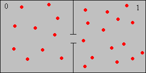
The Ehrenfest chains, named for Paul Ehrenfest, are simple, discrete models for the exchange of gas molecules between two containers. However, they can be formulated as simple ball and urn models; the balls correspond to the molecules and the urns to the two containers. Thus, suppose that we have two urns, labeled 0 and 1, that contain a total of \( m \) balls. The state of the system at time \( n \in \N \) is the number of balls in urn 1, which we will denote by \( X_n \). Our stochastic process is \( \bs{X} = (X_0, X_1, X_2, \ldots) \) with state space \( S = \{0, 1, \ldots, m\} \). Of course, the number of balls in urn 0 at time \( n \) is \( m - X_n \).

The Models

In the basic Ehrenfest model, at each discrete time unit, independently of the past, a ball is selected at random and moved to the other urn.

Figure \(\PageIndex{1}\): The Ehrenfest model

\( \bs{X} \) is a discrete-time Markov chain on \( S \) with transition probability matrix \( P \) given by \[ P(x, x - 1) = \frac{x}{m}, \; P(x, x + 1) = \frac{m - x}{m}, \quad x \in S \]

Proof

We will give a construction of the chain from a more basic process. Let \( V_n \) be the ball selected at time \( n \in \N_+ \). Thus \( \bs{V} = (V_1, V_2, \ldots) \) is a sequence of independent random variables, each uniformly distributed on \( \{1, 2, \ldots, m\} \). Let \( X_0 \in S \) be independent of \( \bs{V} \). (We can start the process any way that we like.) Now define the state process recursively as follows: \[ X_{n+1} = \begin{cases} X_n - 1, & V_{n+1} \le X_n \\ X_n + 1, & V_{n+1} \gt X_n \end{cases}, \quad n \in \N \]

In the Ehrenfest experiment, select the basic model. For selected values of \( m \) and selected values of the initial state, run the chain for 1000 time steps and note the limiting behavior of the proportion of time spent in each state.

Suppose now that we modify the basic Ehrenfest model as follows: at each discrete time, independently of the past, we select a ball at random and a urn at random. We then put the chosen ball in the chosen urn.

\( \bs{X} \) is a discrete-time Markov chain on \( S \) with the transition probability matrix \( Q \) given by \[ Q(x, x - 1) = \frac{x}{2 m}, \; Q(x, x) = \frac{1}{2}, \; Q(x, x + 1) = \frac{m - x}{2 m}, \quad x \in S \]

Proof

Again, we can construct the chain from a more basic process. Let \( X_0 \) and \( \bs{V} \) be as in Theorem 1. Let \( U_n \) be the urn selected at time \( n \in \N_+ \). Thus \( \bs{U} = (U_1, U_2, \ldots) \) is a sequence of independent random variables, each uniformly distributed on \( \{0, 1\} \) (so that \( \bs{U} \) is a fair, Bernoulli trials sequence). Also, \( \bs{U} \) is independent of \( \bs{V} \) and \( X_0 \). Now define the state process recursively as follows: \[ X_{n+1} = \begin{cases} X_n - 1, & V_{n+1} \le X_n, \; U_{n+1} = 0 \\ X_n + 1, & V_{n+1} \gt X_n, \; U_{n+1} = 1 \\ X_n, & \text{otherwise} \end{cases}, \quad n \in \N \]

Note that \( Q(x, y) = \frac{1}{2} P(x, y) \) for \( y \in \{x - 1, x + 1\} \).

In the Ehrenfest experiment, select the modified model. For selected values of \( m \) and selected values of the initial state, run the chain for 1000 time steps and note the limiting behavior of the proportion of time spent in each state.

Classification

The basic and modified Ehrenfest chains are irreducible and positive recurrent.

Proof

The chains are clearly irreducible since every state leads to every other state. It follows that the chains are positive recurrent since the state space \( S \) is finite.

The basic Ehrenfest chain is periodic with period 2. The cyclic classes are the set of even states and the set of odd states. The two-step transition matrix is

\[ P^2(x, x - 2) = \frac{x (x - 1)}{m^2}, \; P^2(x, x) = \frac{x(m - x + 1) + (m - x)(x + 1)}{m^2}, \; P^2(x, x + 2) = \frac{(m - x)(m - x - 1)}{m^2}, \quad x \in S \]

Proof

Note that returns to a state can only occur at even times, so the chain has period 2. The form of \( P^2 \) follows from the formula for \( P \) above.

The modified Ehrenfest chain is aperiodic.

Proof

Note that \( P(x, x) \gt 0 \) for each \( x \in S \).

Invariant and Limiting Distributions

For the basic and modified Ehrenfest chains, the invariant distribution is the binomial distribution with trial parameter \( m \) and success parameter \( \frac{1}{2} \). So the invariant probability density function \( f \) is given by \[ f(x) = \binom{m}{x} \left( \frac{1}{2} \right)^m, \quad x \in S \]

Proof

For the basic chain we have \begin{align*} (f P)(y) & = f(y - 1) P(y - 1, y) + f(y + 1) P(y + 1, y)\\ & = \binom{m}{y - 1} \left(\frac{1}{2}\right)^m \frac{m - y + 1}{m} + \binom{m}{y + 1} \left(\frac{1}{2}\right)^m \frac{y + 1}{m} \\ & = \left(\frac{1}{2}\right)^m \left[\binom{m - 1}{y - 1} + \binom{m - 1}{y}\right] = \left(\frac{1}{2}\right)^m \binom{m}{y} = f(y), \quad y \in S \end{align*} The last step uses a fundamental identity for binomial coefficients. For the modified chain we can use the result for the basic chain: \begin{align*} (f Q)(y) & = f(y - 1) Q(y - 1, y) + f(y) Q(y, y) + f(y + 1)Q(y + 1, y) \\ & = \frac{1}{2} f(y - 1) P(y - 1, y) + \frac{1}{2} f(y + 1) P(y + 1, y) + \frac{1}{2} f(y) = f(y), \quad y \in S \end{align*}

Thus, the invariant distribution corresponds to placing each ball randomly and independently either in urn 0 or in urn 1.

The mean return time to state \( x \in S \) for the basic or modified Ehrenfest chain is \( \mu(x) = 2^m \big/ \binom{m}{x} \).

Proof

This follows from the general theory and the invariant distribution above.

For the basic Ehrenfest chain, the limiting behavior of the chain is as follows:

1. \( P^{2 n}(x, y) \to \binom{m}{y} \left(\frac{1}{2}\right)^{m-1} \) as \( n \to \infty \) if \( x, \, y \in S \) have the same parity (both even or both odd). The limit is 0 otherwise.
2. \( P^{2 n+1}(x, y) \to \binom{m}{y} \left(\frac{1}{2}\right)^{m-1} \) as \( n \to \infty \) if \( x, \, y \in S \) have oppositie parity (one even and one odd). The limit is 0 otherwise.

Proof

These results follow from the general theory and the invariant distribution above, and the fact that the chain is periodic with period 2, with the odd and even integers in \( S \) as the cyclic classes.

For the modified Ehrenfest chain, \( Q^n(x, y) \to \binom{m}{y} \left(\frac{1}{2}\right)^m \) as \( n \to \infty \) for \( x, \, y \in S \).

Proof

Again, this follows from the general theory and the invariant distribution above, and the fact that the chain is aperiodic.

In the Ehrenfest experiment, the limiting binomial distribution is shown graphically and numerically. For each model and for selected values of \( m \) and selected values of the initial state, run the chain for 1000 time steps and note the limiting behavior of the proportion of time spent in each state. How do the choices of \( m \), the initial state, and the model seem to affect the rate of convergence to the limiting distribution?

Reversibility

The basic and modified Ehrenfest chains are reversible.

Proof

Let \( g(x) = \binom{m}{x} \) for \( x \in S \). The crucial observations are \( g(x) P(x, y) = g(y) P(y, x)\) and \(g(x) Q(x, y) = g(y) Q(y, x)\) for all \( x, \, y \in S \). For the basic chain, if \( x \in S \) then \begin{align*} g(x) P(x, x - 1) & = g(x - 1) P(x - 1, x) = \binom{m - 1}{x - 1} \\ g(x) P(x, x + 1) & = g(x + 1) P(x + 1, x) = \binom{m - 1}{x} \end{align*} In all other cases, \( g(x) P(x, y) = g(y) P(y, x) = 0 \). The reversibility condition for the modified chain follows trivially from that of the basic chain since \( Q(x, y) = \frac{1}{2} P(x, y) \) for \( y = x \pm 1 \) (and of course the reversibility condition is trivially satisfied when \( x = y \)). Note that the invariant PDF \( f \) is simply \( g \) normalized. The reversibility condition gives another (and better) proof that \( f \) is invariant.

Run the simulation of the Ehrenfest experiment 10,000 time steps for each model, for selected values of \( m \), and with initial state 0. Note that at first, you can see the arrow of time. After a long period, however, the direction of time is no longer evident.

Computational Exercises

Consider the basic Ehrenfest chain with \( m = 5 \) balls, and suppose that \( X_0 \) has the uniform distribution on \( S \).

1. Compute the probability density function, mean and variance of \( X_1 \).
2. Compute the probability density function, mean and variance of \( X_2 \).
3. Compute the probability density function, mean and variance of \( X_3 \).
4. Sketch the initial probability density function and the probability density functions in parts (a), (b), and (c) on a common set of axes.

Answer

1. \( f_1 = \left( \frac{1}{30}, \frac{7}{30}, \frac{7}{30}, \frac{7}{30}, \frac{7}{30}, \frac{1}{30} \right) \), \( \mu_1 = \frac{5}{2} \), \(\sigma_1^2 = \frac{19}{12} \)
2. \( f_2 = \left( \frac{7}{150}, \frac{19}{150}, \frac{49}{150}, \frac{49}{150}, \frac{19}{150}, \frac{7}{150} \right) \), \( \mu_2 = \frac{5}{2} \), \(\sigma_2^2 = \frac{79}{60} \)
3. \( f_3 = \left( \frac{19}{750}, \frac{133}{750}, \frac{223}{150}, \frac{223}{150}, \frac{133}{150}, \frac{19}{150} \right) \), \( \mu_2 = \frac{5}{2} \), \(\sigma_3^2 = \frac{431}{300} \)

Consider the modified Ehrenfest chain with \( m = 5 \) balls, and suppose that the chain starts in state 2 (with probability 1).

1. Compute the probability density function, mean and standard deviation of \( X_1 \).
2. Compute the probability density function, mean and standard deviation of \( X_2 \).
3. Compute the probability density function, mean and standard deviation of \( X_3 \).
4. Sketch the initial probability density function and the probability density functions in parts (a), (b), and (c) on a common set of axes.

Answer

1. \( f_1 = (0, 0.2, 0.5, 0.3, 0, 0) \), \( \mu_1 = 2.1 \), \(\sigma_1 = 0.7 \)
2. \( f_2 = (0.02, 0.20, 0.42, 0.30, 0.06, 0) \), \( \mu_2 = 2.18 \), \(\sigma_2 = 0.887 \)
3. \( f_3 = (0.030, 0.194, 0.380, 0.300, 0.090, 0.006) \), \( \mu_3 = 2.244 \), \(\sigma_3 = 0.984 \)