11.3: The Geometric Distribution

\(\newcommand{\P}{\mathbb{P}}\) \(\newcommand{\E}{\mathbb{E}}\) \(\newcommand{\R}{\mathbb{R}}\) \(\newcommand{\N}{\mathbb{N}}\) \(\newcommand{\bs}{\boldsymbol}\) \(\newcommand{\var}{\text{var}}\) \(\newcommand{\skw}{\text{skew}}\) \(\newcommand{\kur}{\text{kurt}}\)

Basic Theory

Definitions

Suppose again that our random experiment is to perform a sequence of Bernoulli trials \(\bs{X} = (X_1, X_2, \ldots)\) with success parameter \(p \in (0, 1]\). In this section we will study the random variable \(N\) that gives the trial number of the first success and the random variable \( M \) that gives the number of failures before the first success.

Let \( N = \min\{n \in \N_+: X_n = 1\} \), the trial number of the first success, and let \( M = N - 1 \), the number of failures before the first success. The distribution of \( N \) is the geometric distribution on \( \N_+ \) and the distribution of \( M \) is the geometric distribution on \( \N \). In both cases, \( p \) is the success parameter of the distribution.

Since \( N \) and \( M \) differ by a constant, the properties of their distributions are very similar. Nonetheless, there are applications where it more natural to use one rather than the other, and in the literature, the term geometric distribution can refer to either. In this section, we will concentrate on the distribution of \( N \), pausing occasionally to summarize the corresponding results for \( M \).

The Probability Density Function

\( N \) has probability density function \( f \) given by \(f(n) = p (1 - p)^{n-1}\) for \(n \in \N_+\).

Proof

Note first that \(\{N = n\} = \{X_1 = 0, \ldots, X_{n-1} = 0, X_n = 1\}\). By independence, the probability of this event is \((1 - p)^{n-1} p\).

Check that \( f \) is a valid PDF

By standard results for geometric series \[\sum_{n=1}^\infty \P(N = n) = \sum_{n=1}^\infty (1 - p)^{n-1} p = \frac{p}{1 - (1 - p)} = 1\]

A priori, we might have thought it possible to have \(N = \infty\) with positive probability; that is, we might have thought that we could run Bernoulli trials forever without ever seeing a success. However, we now know this cannot happen when the success parameter \(p\) is positive.

The probability density function of \(M\) is given by \(\P(M = n) = p (1 - p)^n\) for \( n \in \N\).

In the negative binomial experiment, set \(k = 1\) to get the geometric distribution on \(\N_+\). Vary \(p\) with the scroll bar and note the shape and location of the probability density function. For selected values of \(p\), run the simulation 1000 times and compare the relative frequency function to the probability density function.

Note that the probability density functions of \( N \) and \( M \) are decreasing, and hence have modes at 1 and 0, respectively. The geometric form of the probability density functions also explains the term geometric distribution.

Distribution Functions and the Memoryless Property

Suppose that \( T \) is a random variable taking values in \( \N_+ \). Recall that the ordinary distribution function of \( T \) is the function \( n \mapsto \P(T \le n) \). In this section, the complementary function \( n \mapsto \P(T \gt n) \) will play a fundamental role. We will refer to this function as the right distribution function of \( T \). Of course both functions completely determine the distribution of \( T \). Suppose again that \( N \) has the geometric distribution on \( \N_+ \) with success parameter \( p \in (0, 1] \).

\( N \) has right distribution function \( G \) given by \(G(n) = (1 - p)^n\) for \(n \in \N\).

Proof from Bernoulli trials

Note that \(\{N \gt n\} = \{X_1 = 0, \ldots, X_n = 0\}\). By independence, the probability of this event is \((1 - p)^n\).

Direct proof

Using geometric series, \[ \P(N \gt n) = \sum_{k=n+1}^\infty \P(N = k) = \sum_{k=n+1}^\infty (1 - p)^{k-1} p = \frac{p (1 - p)^n}{1 - (1 - p)} = (1 - p)^n \]

From the last result, it follows that the ordinary (left) distribution function of \(N\) is given by \[ F(n) = 1 - (1 - p)^n, \quad n \in \N \] We will now explore another characterization known as the memoryless property.

For \( m \in \N \), the conditional distribution of \(N - m\) given \(N \gt m\) is the same as the distribution of \(N\). That is, \[\P(N \gt n + m \mid N \gt m) = \P(N \gt n); \quad m, \, n \in \N\]

Proof

From the result above and the definition of conditional probability, \[ \P(N \gt n + m \mid N \gt m) = \frac{\P(N \gt n + m)}{\P(N \gt m)} = \frac{(1 - p)^{n+m}}{(1 - p)^m} = (1 - p)^n = \P(N \gt n)\]

Thus, if the first success has not occurred by trial number \(m\), then the remaining number of trials needed to achieve the first success has the same distribution as the trial number of the first success in a fresh sequence of Bernoulli trials. In short, Bernoulli trials have no memory. This fact has implications for a gambler betting on Bernoulli trials (such as in the casino games roulette or craps). No betting strategy based on observations of past outcomes of the trials can possibly help the gambler.

Conversely, if \(T\) is a random variable taking values in \(\N_+\) that satisfies the memoryless property, then \(T\) has a geometric distribution.

Proof

Let \(G(n) = \P(T \gt n)\) for \(n \in \N\). The memoryless property and the definition of conditional probability imply that \(G(m + n) = G(m) G(n)\) for \(m, \; n \in \N\). Note that this is the law of exponents for \(G\). It follows that \(G(n) = G^n(1)\) for \(n \in \N\). Hence \(T\) has the geometric distribution with parameter \(p = 1 - G(1)\).

Moments

Suppose again that \(N\) is the trial number of the first success in a sequence of Bernoulli trials, so that \(N\) has the geometric distribution on \(\N_+\) with parameter \(p \in (0, 1]\). The mean and variance of \(N\) can be computed in several different ways.

\(\E(N) = \frac{1}{p}\)

Proof from the density function

Using the derivative of the geometric series, \begin{align} \E(N) &= \sum_{n=1}^\infty n p (1 - p)^{n-1} = p \sum_{n=1}^\infty n (1 - p)^{n-1} \\ &= p \sum_{n=1}^\infty - \frac{d}{dp}(1 - p)^n = - p \frac{d}{d p} \sum_{n=0}^\infty (1 - p)^n \\ &= -p \frac{d}{dp} \frac{1}{p} = -p \left(-\frac{1}{p^2}\right) = \frac{1}{p}\end{align}

Proof from the right distribution function

Recall that since \( N \) takes positive integer values, its expected value can be computed as the sum of the right distribution function. Hence \[ \E(N) = \sum_{n=0}^\infty \P(N \gt n) = \sum_{n=0}^\infty (1 - p)^n = \frac{1}{p} \]

Proof from Bernoulli trials

We condition on the first trial \( X_1 \): If \( X_1 = 1 \) then \( N = 1 \) and hence \( \E(N \mid X_1 = 1) = 1 \). If \( X_1 = 0 \) (equivalently \( N \gt 1) \) then by the memoryless property, \( N - 1 \) has the same distribution as \( N \). Hence \( \E(N \mid X_1 = 0) = 1 + \E(N) \). In short \[ \E(N \mid X_1) = 1 + (1 - X_1) \E(N) \] It follows that \[ \E(N) = \E\left[\E(N \mid X_1)\right] = 1 + (1 - p) \E(N)\] Solving gives \( \E(N) = \frac{1}{p}\).

This result makes intuitive sense. In a sequence of Bernoulli trials with success parameter \( p \) we would expect to wait \( 1/p \) trials for the first success.

\( \var(N) = \frac{1 - p}{p^2} \)

Direct proof

We first compute \( \E\left[N(N - 1)\right] \). This is an example of a factorial moment, and we will compute the general factorial moments below. Using derivatives of the geometric series again, \begin{align} \E\left[N(N - 1)\right] & = \sum_{n=2}^\infty n (n - 1) p (1 - p)^{n-1} = p (1 - p) \sum_{n=2}^\infty n(n - 1) (1 - p)^{n-2} \\ & = p (1 - p) \frac{d^2}{d p^2} \sum_{n=0}^\infty (1 - p)^n = p (1 - p) \frac{d^2}{dp^2} \frac{1}{p} = p (1 - p) \frac{2}{p^3} = 2 \frac{1 - p}{p^2} \end{align} Since \( \E(N) = \frac{1}{p} \), it follows that \( \E\left(N^2\right) = \frac{2 - p}{p^2} \) and hence \( \var(N) = \frac{1 - p}{p^2} \)

Proof from Bernoulli trials

Recall that \[ \E(N \mid X_1) = 1 + (1 - X_1) \E(N) = 1 + \frac{1}{p} (1 - X_1) \] and by the same reasoning, \( \var(N \mid X_1) = (1 - X_1) \var(N) \). Hence \[ \var(N) = \var\left[\E(N \mid X_1)\right] + \E\left[\var(N \mid X_1)\right] = \frac{1}{p^2} p(1 - p) + (1 - p) \var(N) \] Solving gives \( \var(N) = \frac{1 - p}{p^2} \).

Note that \( \var(N) = 0 \) if \( p = 1 \), hardly surprising since \( N \) is deterministic (taking just the value 1) in this case. At the other extreme, \( \var(N) \uparrow \infty \) as \( p \downarrow 0 \).

In the negative binomial experiment, set \(k = 1\) to get the geometric distribution. Vary \(p\) with the scroll bar and note the location and size of the mean\(\pm\)standard deviation bar. For selected values of \(p\), run the simulation 1000 times and compare the sample mean and standard deviation to the distribution mean and standard deviation.

the probability generating function \( P \) of \(N\) is given by \[ P(t) = \E\left(t^N\right) = \frac{p t}{1 - (1 - p) t}, \quad \left|t\right| \lt \frac{1}{1 - p} \]

Proof

This result follows from yet another application of geometric series: \[ \E\left(t^N\right) = \sum_{n=1}^\infty t^n p (1 - p)^{n-1} = p t \sum_{n=1}^\infty \left[t (1 - p)\right]^{n-1} = \frac{p t}{1 - (1 - p) t}, \quad \left|(1 - p) t\right| \lt 1 \]

Recall again that for \( x \in \R \) and \( k \in \N \), the falling power of \( x \) of order \( k \) is \( x^{(k)} = x (x - 1) \cdots (x - k + 1) \). If \( X \) is a random variable, then \( \E\left[X^{(k)}\right] \) is the factorial moment of \( X \) of order \( k \).

The factorial moments of \(N\) are given by \[ \E\left[N^{(k)}\right] = k! \frac{(1 - p)^{k-1}}{p^k}, \quad k \in \N_+ \]

Proof from geometric series

Using derivatives of geometric series again, \begin{align} \E\left[N^{(k)}\right] & = \sum_{n=k}^\infty n^{(k)} p (1 - p)^{n-1} = p (1 - p)^{k-1} \sum_{n=k}^\infty n^{(k)} (1 - p)^{n-k} \\ & = p (1 - p)^{k-1} (-1)^k \frac{d^k}{dp^k} \sum_{n=0}^\infty (1 - p)^n = p (1 - p)^{k-1} (-1)^k \frac{d^k}{dp^k} \frac{1}{p} = k! \frac{(1 - p)^{k-1}}{p^k} \end{align}

Proof from the generating function

Recall that \(\E\left[N^{(k)}\right] = P^{(k)}(1)\) where \(P\) is the probability generating function of \(N\). So the result follows from standard calculus.

Suppose that \( p \in (0, 1) \). The skewness and kurtosis of \(N\) are

1. \(\skw(N) = \frac{2 - p}{\sqrt{1 - p}}\)
2. \(\kur(N) = \frac{p^2}{1 - p}\)

Proof

The factorial moments can be used to find the moments of \(N\) about 0. The results then follow from the standard computational formulas for skewness and kurtosis.

Note that the geometric distribution is always positively skewed. Moreover, \( \skw(N) \to \infty \) and \( \kur(N) \to \infty \) as \( p \uparrow 1 \).

Suppose now that \(M = N - 1\), so that \(M\) (the number of failures before the first success) has the geometric distribution on \(\N\). Then

1. \(\E(M) = \frac{1 - p}{p}\)
2. \(\var(M) = \frac{1 - p}{p^2}\)
3. \(\skw(M) = \frac{2 - p}{\sqrt{1 - p}}\)
4. \(\kur(M) = \frac{p^2}{1 - p}\)
5. \(\E\left(t^M\right) = \frac{p}{1 - (1 - p) \, t}\) for \(\left|t\right| \lt \frac{1}{1 - p}\)

Of course, the fact that the variance, skewness, and kurtosis are unchanged follows easily, since \(N\) and \(M\) differ by a constant.

The Quantile Function

Let \(F\) denote the distribution function of \(N\), so that \(F(n) = 1 - (1 - p)^n\) for \(n \in \N\). Recall that \(F^{-1}(r) = \min \{n \in \N_+: F(n) \ge r\}\) for \(r \in (0, 1)\) is the quantile function of \(N\).

The quantile function of \(N\) is \[ F^{-1}(r) = \left\lceil \frac{\ln(1 - r)}{\ln(1 - p)}\right\rceil, \quad r \in (0, 1) \]

Of course, the quantile function, like the probability density function and the distribution function, completely determines the distribution of \(N\). Moreover, we can compute the median and quartiles to get measures of center and spread.

The first quartile, the median (or second quartile), and the third quartile are

1. \(F^{-1}\left(\frac{1}{4}\right) = \left\lceil \ln(3/4) \big/ \ln(1 - p)\right\rceil \approx \left\lceil-0.2877 \big/ \ln(1 - p)\right\rceil\)
2. \(F^{-1}\left(\frac{1}{2}\right) = \left\lceil \ln(1/2) \big/ \ln(1 - p)\right\rceil \approx \left\lceil-0.6931 \big/ \ln(1 - p)\right\rceil\)
3. \(F^{-1}\left(\frac{3}{4}\right) = \left\lceil \ln(1/4) \big/ \ln(1 - p)\right\rceil \approx \left\lceil-1.3863 \big/ \ln(1 - p)\right\rceil\)

Open the special distribution calculator, and select the geometric distribution and CDF view. Vary \( p \) and note the shape and location of the CDF/quantile function. For various values of \( p \), compute the median and the first and third quartiles.

The Constant Rate Property

Suppose that \(T\) is a random variable taking values in \(\N_+\), which we interpret as the first time that some event of interest occurs.

The function \( h \) given by \[ h(n) = \P(T = n \mid T \ge n) = \frac{\P(T = n)}{\P(T \ge n)}, \quad n \in \N_+ \] is the rate function of \(T\).

If \(T\) is interpreted as the (discrete) lifetime of a device, then \(h\) is a discrete version of the failure rate function studied in reliability theory. However, in our usual formulation of Bernoulli trials, the event of interest is success rather than failure (or death), so we will simply use the term rate function to avoid confusion. The constant rate property characterizes the geometric distribution. As usual, let \(N\) denote the trial number of the first success in a sequence of Bernoulli trials with success parameter \(p \in (0, 1)\), so that \(N\) has the geometric distribution on \(\N_+\) with parameter \(p\).

\(N\) has constant rate \(p\).

Proof

From the results above, \( \P(N = n) = p (1 - p)^{n-1} \) and \( \P(N \ge n) = \P(N \gt n - 1) = (1 - p)^{n-1} \), so \( \P(N = n) \big/ \P(N \ge n) = p \) for \( n \in \N_+ \).

Conversely, if \(T\) has constant rate \(p \in (0, 1)\) then \(T\) has the geometric distrbution on \(\N_+\) with success parameter \(p\).

Proof

Let \(H(n) = \P(T \ge n)\) for \(n \in \N_+\). From the constant rate property, \(\P(T = n) = p \, H(n)\) for \(n \in \N_+\). Next note that \(\P(T = n) = H(n) - H(n + 1)\) for \(n \in \N_+\). Thus, \(H\) satisfies the recurrence relation \(H(n + 1) = (1 - p) \, H(n)\) for \(n \in \N_+\). Also \(H\) satisfies the initial condition \(H(1) = 1\). Solving the recurrence relation gives \(H(n) = (1 - p)^{n-1}\) for \(n \in \N_+\).

Relation to the Uniform Distribution

Suppose again that \( \bs{X} = (X_1, X_2, \ldots) \) is a sequence of Bernoulli trials with success parameter \( p \in (0, 1) \). For \( n \in \N_+ \), recall that \(Y_n = \sum_{i=1}^n X_i\), the number of successes in the first \(n\) trials, has the binomial distribution with parameters \(n\) and \(p\). As before, \( N \) denotes the trial number of the first success.

Suppose that \( n \in \N_+ \). The conditional distribution of \(N\) given \(Y_n = 1\) is uniform on \(\{1, 2, \ldots, n\}\).

Proof from sampling

We showed in the last section that given \( Y_n = k \), the trial numbers of the successes form a random sample of size \( k \) chosen without replacement from \( \{1, 2, \ldots, n\} \). This result is a simple corollary with \( k = 1 \)

Direct proof

For \( j \in \{1, 2, \ldots, n\} \) \[ \P(N = j \mid Y_n = 1) = \frac{\P(N = j, Y_n = 1)}{\P(Y_n = 1)} = \frac{\P\left(Y_{j-1} = 0, X_j = 1, Y_{n} - Y_j = 0\right)}{\P(Y_n = 1)} \] In words, the events in the numerator of the last fraction are that there are no successes in the first \( j - 1 \) trials, a success on trial \( j \), and no successes in trials \( j + 1 \) to \( n \). These events are independent so \[ \P(N = j \mid Y_n = 1) = \frac{(1 - p)^{j-1} p (1 - p)^{n-j}}{n p (1 - p)^{n - 1}} = \frac{1}{n}\]

Note that the conditional distribution does not depend on the success parameter \(p\). If we know that there is exactly one success in the first \(n\) trials, then the trial number of that success is equally likely to be any of the \(n\) possibilities.

Another connection between the geometric distribution and the uniform distribution is given below in the alternating coin tossing game: the conditional distribution of \( N \) given \( N \le n \) converges to the uniform distribution on \( \{1, 2, \ldots, n\} \) as \( p \downarrow 0 \).

Relation to the Exponential Distribution

The Poisson process on \( [0, \infty) \), named for Simeon Poisson, is a model for random points in continuous time. There are many deep and interesting connections between the Bernoulli trials process (which can be thought of as a model for random points in discrete time) and the Poisson process. These connections are explored in detail in the chapter on the Poisson process. In this section we just give the most famous and important result—the convergence of the geometric distribution to the exponential distribution. The geometric distribution, as we know, governs the time of the first random point in the Bernoulli trials process, while the exponential distribution governs the time of the first random point in the Poisson process.

For reference, the exponential distribution with rate parameter \( r \in (0, \infty) \) has distribution function \( F(x) = 1 - e^{-r x} \) for \( x \in [0, \infty) \). The mean of the exponential distribution is \( 1 / r \) and the variance is \( 1 / r^2 \). In addition, the moment generating function is \( s \mapsto \frac{1}{s - r} \) for \( s \gt r \).

For \( n \in \N_+ \), suppose that \( U_n \) has the geometric distribution on \( \N_+ \) with success parameter \( p_n \in (0, 1) \), where \( n p_n \to r \gt 0 \) as \( n \to \infty \). Then the distribution of \( U_n / n \) converges to the exponential distribution with parameter \( r \) as \( n \to \infty \).

Proof

Let \( F_n \) denote the CDF of \( U_n / n \). Then for \( x \in [0, \infty) \) \[ F_n(x) = \P\left(\frac{U_n}{n} \le x\right) = \P(U_n \le n x) = \P\left(U_n \le \lfloor n x \rfloor\right) = 1 - \left(1 - p_n\right)^{\lfloor n x \rfloor} \] But by a famous limit from calculus, \( \left(1 - p_n\right)^n = \left(1 - \frac{n p_n}{n}\right)^n \to e^{-r} \) as \( n \to \infty \), and hence \( \left(1 - p_n\right)^{n x} \to e^{-r x} \) as \( n \to \infty \). But by definition, \( \lfloor n x \rfloor \le n x \lt \lfloor n x \rfloor + 1\) or equivalently, \( n x - 1 \lt \lfloor n x \rfloor \le n x \) so it follows that \( \left(1 - p_n \right)^{\lfloor n x \rfloor} \to e^{- r x} \) as \( n \to \infty \). Hence \( F_n(x) \to 1 - e^{-r x} \) as \( n \to \infty \), which is the CDF of the exponential distribution.

Note that the condition \( n p_n \to r \) as \( n \to \infty \) is the same condition required for the convergence of the binomial distribution to the Poisson that we studied in the last section.

Special Families

The geometric distribution on \( \N \) is an infinitely divisible distribution and is a compound Poisson distribution. For the details, visit these individual sections and see the next section on the negative binomial distribution.

Examples and Applications

Simple Exercises

A standard, fair die is thrown until an ace occurs. Let \(N\) denote the number of throws. Find each of the following:

1. The probability density function of \(N\).
2. The mean of \(N\).
3. The variance of \(N\).
4. The probability that the die will have to be thrown at least 5 times.
5. The quantile function of \(N\).
6. The median and the first and third quartiles.

Answwer

1. \(\P(N = n) = \left(\frac{5}{6}\right)^{n-1} \frac{1}{6}\) for \( n \in \N_+\)
2. \(\E(N) = 6\)
3. \(\var(N) = 30\)
4. \(\P(N \ge 5) = 525 / 1296\)
5. \(F^{-1}(r) = \lceil \ln(1 - r) / \ln(5 / 6)\rceil\) for \( r \in (0, 1)\)
6. Quartiles \(q_1 = 2\), \(q_2 = 4\), \(q_3 = 8\)

A type of missile has failure probability 0.02. Let \(N\) denote the number of launches before the first failure. Find each of the following:

1. The probability density function of \(N\).
2. The mean of \(N\).
3. The variance of \(N\).
4. The probability of 20 consecutive successful launches.
5. The quantile function of \(N\).
6. The median and the first and third quartiles.

Answer

1. \(\P(N = n) \ \left(\frac{49}{50}\right)^{n-1} \frac{1}{50}\) for \( n \in \N_+\)
2. \(\E(N) = 50\)
3. \(\var(N) = 2450\)
4. \(\P(N \gt 20) = 0.6676\)
5. \(F^{-1}(r) = \lceil \ln(1 - r) / \ln(0.98)\rceil\) for \( r \in (0, 1)\)
6. Quartiles \(q_1 = 15\), \(q_2 = 35\), \(q_3 = 69\)

A student takes a multiple choice test with 10 questions, each with 5 choices (only one correct). The student blindly guesses and gets one question correct. Find the probability that the correct question was one of the first 4.

Answer

0.4

Recall that an American roulette wheel has 38 slots: 18 are red, 18 are black, and 2 are green. Suppose that you observe red or green on 10 consecutive spins. Give the conditional distribution of the number of additional spins needed for black to occur.

Answer

Geometric with \(p = \frac{18}{38}\)

The game of roulette is studied in more detail in the chapter on Games of Chance.

In the negative binomial experiment, set \(k = 1\) to get the geometric distribution and set \(p = 0.3\). Run the experiment 1000 times. Compute the appropriate relative frequencies and empirically investigate the memoryless property \[ \P(V \gt 5 \mid V \gt 2) = \P(V \gt 3) \]

The Petersburg Problem

We will now explore a gambling situation, known as the Petersburg problem, which leads to some famous and surprising results. Suppose that we are betting on a sequence of Bernoulli trials with success parameter \(p \in (0, 1)\). We can bet any amount of money on a trial at even stakes: if the trial results in success, we receive that amount, and if the trial results in failure, we must pay that amount. We will use the following strategy, known as a martingale strategy:

1. We bet \(c\) units on the first trial.
2. Whenever we lose a trial, we double the bet for the next trial.
3. We stop as soon as we win a trial.

Let \( N \) denote the number of trials played, so that \( N \) has the geometric distribution with parameter \( p \), and let \( W \) denote our net winnings when we stop.

\(W = c\)

Proof

The first win occurs on trial \(N\), so the initial bet was doubled \(N - 1\) times. The net winnings are \[W = -c \sum_{i=0}^{N-2} 2^i + c 2^{N-1} = c\left(1 - 2^{N-1} + 2^{N-1}\right) = c\]

Thus, \(W\) is not random and \(W\) is independent of \(p\)! Since \(c\) is an arbitrary constant, it would appear that we have an ideal strategy. However, let us study the amount of money \(Z\) needed to play the strategy.

\(Z = c (2^N - 1)\)

The expected amount of money needed for the martingale strategy is \[ \E(Z) = \begin{cases} \frac{c}{2 p - 1}, & p \gt \frac{1}{2} \\ \infty, & p \le \frac{1}{2} \end{cases} \]

Thus, the strategy is fatally flawed when the trials are unfavorable and even when they are fair, since we need infinite expected capital to make the strategy work in these cases.

Compute \(\E(Z)\) explicitly if \(c = 100\) and \(p = 0.55\).

Answer

$1000

In the negative binomial experiment, set \(k = 1\). For each of the following values of \(p\), run the experiment 100 times. For each run compute \(Z\) (with \(c = 1\)). Find the average value of \(Z\) over the 100 runs:

1. \(p = 0.2\)
2. \(p = 0.5\)
3. \(p = 0.8\)

For more information about gambling strategies, see the section on Red and Black. Martingales are studied in detail in a separate chapter.

The Alternating Coin-Tossing Game

A coin has probability of heads \(p \in (0, 1]\). There are \(n\) players who take turns tossing the coin in round-robin style: player 1 first, then player 2, continuing until player \(n\), then player 1 again, and so forth. The first player to toss heads wins the game.

Let \(N\) denote the number of the first toss that results in heads. Of course, \(N\) has the geometric distribution on \(\N_+\) with parameter \(p\). Additionally, let \(W\) denote the winner of the game; \(W\) takes values in the set \(\{1, 2, \ldots, n\}\). We are interested in the probability distribution of \(W\).

For \(i \in \{1, 2, \ldots, n\}\), \(W = i\) if and only if \(N = i + k n\) for some \(k \in \N\). That is, using modular arithmetic, \[ W = [(N - 1) \mod n] + 1 \]

The winning player \(W\) has probability density function \[ \P(W = i) = \frac{p (1 - p)^{i-1}}{1 - (1 - p)^n}, \quad i \in \{1, 2, \ldots, n\} \]

Proof

This follows from the previous exercise and the geometric distribution of \(N\).

\(\P(W = i) = (1 - p)^{i-1} \P(W = 1)\) for \(i \in \{1, 2, \ldots, n\}\).

Proof

This result can be argued directly, using the memoryless property of the geometric distribution. In order for player \(i\) to win, the previous \(i - 1\) players must first all toss tails. Then, player \(i\) effectively becomes the first player in a new sequence of tosses. This result can be used to give another derivation of the probability density function in the previous exercise.

Note that \(\P(W = i)\) is a decreasing function of \(i \in \{1, 2, \ldots, n\}\). Not surprisingly, the lower the toss order the better for the player.

Explicitly compute the probability density function of \(W\) when the coin is fair (\(p = 1 / 2\)).

Answer

\(\P(W = i) = 2^{n-1} \big/ (2^n - 1), \quad i \in \{1, 2, \ldots, n\}\)

Note from the result above that \(W\) itself has a truncated geometric distribution.

The distribution of \(W\) is the same as the conditional distribution of \(N\) given \(N \le n\): \[ \P(W = i) = \P(N = i \mid N \le n), \quad i \in \{1, 2, \ldots, n\} \]

The following problems explore some limiting distributions related to the alternating coin-tossing game.

For fixed \(p \in (0, 1]\), the distribution of \(W\) converges to the geometric distribution with parameter \(p\) as \(n \uparrow \infty\).

For fixed \(n\), the distribution of \(W\) converges to the uniform distribution on \(\{1, 2, \ldots, n\}\) as \(p \downarrow 0\).

Players at the end of the tossing order should hope for a coin biased towards tails.

Odd Man Out

In the game of odd man out, we start with a specified number of players, each with a coin that has the same probability of heads. The players toss their coins at the same time. If there is an odd man, that is a player with an outcome different than all of the other players, then the odd player is eliminated; otherwise no player is eliminated. In any event, the remaining players continue the game in the same manner. A slight technical problem arises with just two players, since different outcomes would make both players odd. So in this case, we might (arbitrarily) make the player with tails the odd man.

Suppose there are \(k \in \{2, 3, \ldots\}\) players and \(p \in [0, 1]\). In a single round, the probability of an odd man is \[r_k(p) = \begin{cases} 2 p (1 - p), & k = 2 \\ k p (1 - p)^{k-1} + k p^{k-1} (1 - p), & k \in \{3, 4, \ldots\} \end{cases}\]

Proof

Let \(Y\) denote the number of heads. If \(k = 2\), the event that there is an odd man is \(\{Y = 1\}\). If \(k \ge 3\), the event that there is an odd man is \(\{Y \in \{1, k - 1\}\}\). The result now follows since \(Y\) has a binomial distribution with parameters \( k \) and \( p \).

The graph of \(r_k\) is more interesting than you might think.

Figure \(\PageIndex{1}\): The graphs of \( r_k \) for \( k \in \{3, 4, 5, 6\} \)

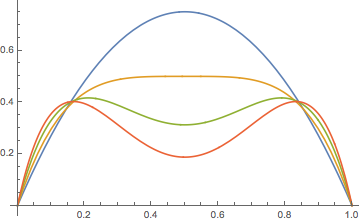
For \( k \in \{2, 3, \ldots\} \), \(r_k\) has the following properties:

1. \(r_k(0) = r_k(1) = 0\)
2. \(r_k\) is symmetric about \(p = \frac{1}{2}\)
3. For fixed \(p \in [0, 1]\), \(r_k(p) \to 0\) as \(k \to \infty\).

Proof

These properties are clear from the functional form of \( r_k(p) \). Note that \( r_k(p) = r_k(1 - p) \).

For \( k \in \{2, 3, 4\} \), \(r_k\) has the following properties:

1. \( r_k \) increases and then decreases, with maximum at \(p = \frac{1}{2}\).
2. \( r_k \) is concave downward

Proof

This follows by computing the first derivatives: \(r_2^\prime(p) = 2 (1 - 2 p)\), \(r_3^\prime(p) = 3 (1 - 2 p)\), \(r_4^\prime(p) = 4 (1 - 2 p)^3\), and the second derivatives: \( r_2^{\prime\prime}(p) = -4 \), \( r_3^{\prime\prime}(p) = - 6 \), \( r_4^{\prime\prime}(p) = -24 (1 - 2 p)^2 \).

For \( k \in \{5, 6, \ldots\} \), \(r_k\) has the following properties:

1. The maximum occurs at two points of the form \(p_k\) and \(1 - p_k\) where \( p_k \in \left(0, \frac{1}{2}\right) \) and \(p_k \to 0\) as \(k \to \infty\).
2. The maximum value \(r_k(p_k) \to 1/e \approx 0.3679\) as \(k \to \infty\).
3. The graph has a local minimum at \(p = \frac{1}{2}\).

Proof sketch

Note that \(r_k(p) = s_k(p) + s_k(1 - p)\) where \(s_k(t) = k t^{k-1}(1 - t)\) for \(t \in [0, 1]\). Also, \(p \mapsto s_k(p)\) is the dominant term when \(p \gt \frac{1}{2}\) while \(p \mapsto s_k(1 - p)\) is the dominant term when \(p \lt \frac{1}{2}\). A simple analysis of the derivative shows that \(s_k\) increases and then decreases, reaching its maximum at \((k - 1) / k\). Moreover, the maximum value is \(s_k\left[(k - 1) / k\right] = (1 - 1 / k)^{k-1} \to e^{-1}\) as \(k \to \infty\). Also, \( s_k \) is concave upward and then downward, wit inflection point at \( (k - 2) / k \).

Suppose \(p \in (0, 1)\), and let \(N_k\) denote the number of rounds until an odd man is eliminated, starting with \(k\) players. Then \(N_k\) has the geometric distribution on \(\N_+\) with parameter \(r_k(p)\). The mean and variance are

1. \(\mu_k(p) = 1 \big/ r_k(p)\)
2. \(\sigma_k^2(p) = \left[1 - r_k(p)\right] \big/ r_k^2(p)\)

As we might expect, \(\mu_k(p) \to \infty\) and \(\sigma_k^2(p) \to \infty\) as \(k \to \infty\) for fixed \(p \in (0, 1)\). On the other hand, from the result above, \(\mu_k(p_k) \to e\) and \(\sigma_k^2(p_k) \to e^2 - e\) as \(k \to \infty\).

Suppose we start with \(k \in \{2, 3, \ldots\}\) players and \(p \in (0, 1)\). The number of rounds until a single player remains is \(M_k = \sum_{j = 2}^k N_j\) where \((N_2, N_3, \ldots, N_k)\) are independent and \(N_j\) has the geometric distribution on \(\N_+\) with parameter \(r_j(p)\). The mean and variance are

1. \(\E(M_k) = \sum_{j=2}^k 1 \big/ r_j(p)\)
2. \(\var(M_k) = \sum_{j=2}^k \left[1 - r_j(p)\right] \big/ r_j^2(p)\)

Proof

The form of \(M_k\) follows from the previous result: \(N_k\) is the number of rounds until the first player is eliminated. Then the game continues independently with \(k - 1\) players, so \(N_{k-1}\) is the number of additional rounds until the second player is eliminated, and so forth. Parts (a) and (b) follow from the previous result and standard properties of expected value and variance.

Starting with \(k\) players and probability of heads \(p \in (0, 1)\), the total number of coin tosses is \(T_k = \sum_{j=2}^k j N_j\). The mean and variance are

1. \(\E(T_k) = \sum_{j=2}^k j \big/ r_j(p)\)
2. \(\var(T_k) = \sum_{j=2}^k j^2 \left[1 - r_j(p)\right] \big/ r_j^2(p)\)

Proof

As before, the form of \(M_k\) follows from result above: \(N_k\) is the number of rounds until the first player is eliminated, and each these rounds has \(k\) tosses. Then the game continues independently with \(k - 1\) players, so \(N_{k-1}\) is the number of additional rounds until the second player is eliminated with each round having \(k - 1\) tosses, and so forth. Parts (a) and (b) also follow from the result above and standard properties of expected value and variance.

Number of Trials Before a Pattern

Consider again a sequence of Bernoulli trials \( \bs X = (X_1, X_2, \ldots) \) with success parameter \( p \in (0, 1) \). Recall that the number of trials \( M \) before the first success (outcome 1) occurs has the geometric distribution on \( \N \) with parameter \( p \). A natural generalization is the random variable that gives the number of trials before a specific finite sequence of outcomes occurs for the first time. (Such a sequence is sometimes referred to as a word from the alphabet \( \{0, 1\} \) or simply a bit string). In general, finding the distribution of this variable is a difficult problem, with the difficulty depending very much on the nature of the word. The problem of finding just the expected number of trials before a word occurs can be solved using powerful tools from the theory of renewal processes and from the theory of martingalges.

To set up the notation, let \( \bs x \) denote a finite bit string and let \( M_{\bs x} \) denote the number of trials before \( \bs x \) occurs for the first time. Finally, let \( q = 1 - p \). Note that \( M_{\bs x} \) takes values in \( \N \). In the following exercises, we will consider \( \bs x = 10 \), a success followed by a failure. As always, try to derive the results yourself before looking at the proofs.

The probability density function \( f_{10} \) of \( M_{10} \) is given as follows:

1. If \( p \ne \frac{1}{2} \) then \[ f_{10}(n) = p q \frac{p^{n+1} - q^{n+1}}{p - q}, \quad n \in \N \]
2. If \(p = \frac{1}{2}\) then \( f_{10}(n) = (n + 1) \left(\frac{1}{2}\right)^{n+2} \) for \( n \in \N \).

Proof

For \( n \in \N \), the event \(\{M_{10} = n\}\) can only occur if there is an initial string of 0s of length \( k \in \{0, 1, \ldots, n\} \) followed by a string of 1s of length \( n - k \) and then 1 on trial \( n + 1 \) and 0 on trial \( n + 2 \). Hence \[ f_{10}(n) = \P(M_{10} = n) = \sum_{k=0}^n q^k p^{n - k} p q, \quad n \in \N \] The stated result then follows from standard results on geometric series.

It's interesting to note that \( f \) is symmetric in \( p \) and \( q \), that is, symmetric about \( p = \frac{1}{2} \). It follows that the distribution function, probability generating function, expected value, and variance, which we consider below, are all also symmetric about \( p = \frac{1}{2} \). It's also interesting to note that \( f_{10}(0) = f_{10}(1) = p q \), and this is the largest value. So regardless of \( p \in (0, 1) \) the distribution is bimodal with modes 0 and 1.

The distribution function \( F_{10} \) of \( M_{10} \) is given as follows:

1. If \( p \ne \frac{1}{2} \) then \[ F_{10}(n) = 1 - \frac{p^{n+3} - q^{n+3}}{p - q}, \quad n \in \N \]
2. If \( p = \frac{1}{2} \) then \( F_{10} = 1 - (n + 3) \left(\frac{1}{2}\right)^{n+2} \) for \( n \in \N \).

Proof

By definition, \(F_{10}(n) = \sum_{k=0}^n f_{10}(k)\) for \( n \in \N \). The stated result then follows from the previous theorem, standard results on geometric series, and some algebra.

The probability generating function \( P_{10} \) of \( M_{10} \) is given as follows:

1. If \( p \ne \frac{1}{2} \) then \[ P_{10}(t) = \frac{p q}{p - q} \left(\frac{p}{1 - t p} - \frac{q}{1 - t q}\right), \quad |t| \lt \min \{1 / p, 1 / q\} \]
2. If \( p = \frac{1}{2} \) then \(P_{10}(t) = 1 / (t - 2)^2\) for \( |t| \lt 2 \)

Proof

By definition, \[ P_{10}(t) = \E\left(t^{M_{10}}\right) = \sum_{n=0}^\infty f_{10}(n) t^n \] for all \( t \in \R \) for which the series converges absolutely. The stated result then follows from the theorem above, and once again, standard results on geometric series.

The mean of \( M_{10} \) is given as follows:

1. If \( p \ne \frac{1}{2} \) then \[ \E(M_{10}) = \frac{p^4 - q^4}{p q (p - q)} \]
2. If \( p = \frac{1}{2} \) then \( \E(M_{10}) = 2 \).

Proof

Recall that \( \E(M_{10}) = P^\prime_{10}(1) \) so the stated result follows from calculus, using the previous theorem on the probability generating function. The mean can also be computed from the definition \( \E(M_{10}) = \sum_{n=0}^\infty n f_{10}(n) \) using standard results from geometric series, but this method is more tedious.

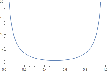
The graph of \( \E(M_{10}) \) as a function of \( p \in (0, 1) \) is given below. It's not surprising that \( \E(M_{10}) \to \infty \) as \( p \downarrow 0 \) and as \( p \uparrow 1 \), and that the minimum value occurs when \( p = \frac{1}{2} \).

Figure \(\PageIndex{2}\): \( \E(M_{10}) \) as a function of \( p \)

The variance of \( M_{10} \) is given as follows:

1. If \( p \ne \frac{1}{2} \) then \[ \var(M_{10}) = \frac{2}{p^2 q^2} \left(\frac{p^6 - q^6}{p - q}\right) + \frac{1}{p q} \left(\frac{p^4 - q^4}{p - q}\right) - \frac{1}{p^2 q^2}\left(\frac{p^4 - q^4}{p - q}\right)^2 \]
2. If \( p = \frac{1}{2} \) then \( \var(M_{10}) = 4 \).

Proof

Recall that \( P^{\prime \prime}_{10}(1) = \E[M_{10}(M_{10} - 1)] \), the second factorial moment, and so \[ \var(M_{10}) = P^{\prime \prime}_{10}(1) + P^\prime_{10}(1) - [P^\prime_{10}(1)]^2 \] The stated result then follows from calculus and the theorem above giving the probability generating function.