4.2: Additional Properties

\(\renewcommand{\P}{\mathbb{P}}\) \(\newcommand{\E}{\mathbb{E}}\) \(\newcommand{\R}{\mathbb{R}}\) \(\newcommand{\N}{\mathbb{N}}\) \(\newcommand{\bs}{\boldsymbol}\)

In this section, we study some properties of expected value that are a bit more specialized than the basic properties considered in the previous section. Nonetheless, the new results are also very important. They include two fundamental inequalities as well as special formulas for the expected value of a nonnegative variable. As usual, unless otherwise noted, we assume that the referenced expected values exist.

Basic Theory

Markov's Inequality

Our first result is known as Markov's inequality (named after Andrei Markov). It gives an upper bound for the tail probability of a nonnegative random variable in terms of the expected value of the variable.

If \(X\) is a nonnegative random variable, then \[ \P(X \ge x) \le \frac{\E(X)}{x}, \quad x \gt 0 \]

Proof

For \( x \gt 0 \), note that \(x \cdot \bs{1}(X \ge x) \le X\). Taking expected values through this inequality gives \(x \P(X \ge x) \le \E(X)\).

The upper bound in Markov's inequality may be rather crude. In fact, it's quite possible that \( \E(X) \big/ x \ge 1 \), in which case the bound is worthless. However, the real value of Markov's inequality lies in the fact that it holds with no assumptions whatsoever on the distribution of \( X \) (other than that \( X \) be nonnegative). Also, as an example below shows, the inequality is tight in the sense that equality can hold for a given \( x \). Here is a simple corollary of Markov's inequality.

If \( X \) is a real-valued random variable and \( k \in (0, \infty) \) then \[ \P(\left|X\right| \ge x) \le \frac{\E\left(\left|X\right|^k\right)}{x^k} \quad x \gt 0 \]

Proof

Since \( k \ge 0 \), the function \( x \mapsto x^k \) is strictly increasing on \( [0, \infty) \). Hence using Markov's inequality, \[ \P(\left|X\right| \ge x) = \P\left(\left|X\right|^k \ge x^k\right) \le \frac{\E\left(\left|X\right|^k\right)}{x^k} \]

In this corollary of Markov's inequality, we could try to find \( k \gt 0 \) so that \( \E\left( \left|X\right|^k\right) \big/ x^k \) is minimized, thus giving the tightest bound on \( \P\left(\left|X\right|\right) \ge x)\).

Right Distribution Function

Our next few results give alternative ways to compute the expected value of a nonnegative random variable by means of the right-tail distribution function. This function also known as the reliability function if the variable represents the lifetime of a device.

If \(X\) is a nonnegative random variable then \[ \E(X) = \int_0^\infty \P(X \gt x) \, dx \]

Proof

A proof can be constructed by expressing \(\P(X \gt x)\) in terms of the probability density function of \(X\), as a sum in the discrete case or an integral in the continuous case. Then in the expression \( \int_0^\infty \P(X \gt x) \, dx \) interchange the integral and the sum (in the discrete case) or the two integrals (in the continuous case). There is a much more elegant proof if we use the fact that we can interchange expected values and integrals when the integrand is nonnegative: \[ \int_0^\infty \P(X \gt x) \, dx = \int_0^\infty \E\left[\bs{1}(X \gt x)\right] \, dx = \E \left(\int_0^\infty \bs{1}(X \gt x) \, dx \right) = \E\left( \int_0^X 1 \, dx \right) = \E(X) \] This interchange is a special case of Fubini's theorem, named for the Italian mathematician Guido Fubini. See the advanced section on expected value as an integral for more details.

Here is a slightly more general result:

If \( X \) is a nonnegative random variable and \( k \in (0, \infty) \) then \[ \E(X^k) = \int_0^\infty k x^{k-1} \P(X \gt x) \, dx \]

Proof

The same basic proof works: \[ \int_0^\infty k x^{k-1} \P(X \gt x) \, dx = \int_0^\infty k x^{k-1} \E\left[\bs{1}(X \gt x)\right] \, dx = \E \left(\int_0^\infty k x^{k-1} \bs{1}(X \gt x) \, dx \right) = \E\left( \int_0^X k x^{k-1} \, dx \right) = \E(X^k) \]

The following result is similar to the theorem above, but is specialized to nonnegative integer valued variables:

Suppose that \(N\) has a discrete distribution, taking values in \(\N\). Then \[ \E(N) = \sum_{n=0}^\infty \P(N \gt n) = \sum_{n=1}^\infty \P(N \ge n) \]

Proof

First, the two sums on the right are equivalent by a simple change of variables. A proof can be constructed by expressing \(\P(N \gt n)\) as a sum in terms of the probability density function of \(N\). Then in the expression \( \sum_{n=0}^\infty \P(N \gt n) \) interchange the two sums. Here is a more elegant proof: \[ \sum_{n=1}^\infty \P(N \ge n) = \sum_{n=1}^\infty \E\left[\bs{1}(N \ge n)\right] = \E\left(\sum_{n=1}^\infty \bs{1}(N \ge n) \right) = \E\left(\sum_{n=1}^N 1 \right) = \E(N) \] This interchange is a special case of a general rule that allows the interchange of expected value and an infinite series, when the terms are nonnegative. See the advanced section on expected value as an integral for more details.

A General Definition

The special expected value formula for nonnegative variables can be used as the basis of a general formulation of expected value that would work for discrete, continuous, or even mixed distributions, and would not require the assumption of the existence of probability density functions. First, the special formula is taken as the definition of \(\E(X)\) if \(X\) is nonnegative.

If \( X \) is a nonnegative random variable, define \[ \E(X) = \int_0^\infty \P(X \gt x) \, dx \]

Next, for \(x \in \R\), recall that the positive and negative parts of \(x\) are \( x^+ = \max\{x, 0\}\) and \(x^- = \max\{0, -x\} \).

For \(x \in \R\),

1. \(x^+ \ge 0\), \(x^- \ge 0\)
2. \(x = x^+ - x^-\)
3. \(\left|x\right| = x^+ + x^-\)

Now, if \(X\) is a real-valued random variable, then \(X^+\) and \(X^-\), the positive and negative parts of \(X\), are nonnegative random variables, so their expected values are defined as above. The definition of \( \E(X) \) is then natural, anticipating of course the linearity property.

If \( X \) is a real-valued random variable, define \(\E(X) = \E\left(X^+\right) - \E\left(X^-\right)\), assuming that at least one of the expected values on the right is finite.

The usual formulas for expected value in terms of the probability density function, for discrete, continuous, or mixed distributions, would now be proven as theorems. We will not go further in this direction, however, since the most complete and general definition of expected value is given in the advanced section on expected value as an integral.

The Change of Variables Theorem

Suppose that \( X \) takes values in \( S \) and has probability density function \( f \). Suppose also that \( r: S \to \R \), so that \( r(X) \) is a real-valued random variable. The change of variables theorem gives a formula for computing \( \E\left[r(X)\right] \) without having to first find the probability density function of \( r(X) \). If \( S \) is countable, so that \( X \) has a discrete distribution, then \[ \E\left[r(X)\right] = \sum_{x \in S} r(x) f(x) \] If \( S \subseteq \R^n \) and \( X \) has a continuous distribution on \( S \) then \[ \E\left[r(X)\right] = \int_S r(x) f(x) \, dx \] In both cases, of course, we assume that the expected values exist. In the previous section on basic properties, we proved the change of variables theorem when \( X \) has a discrete distribution and when \( X \) has a continuous distribution but \( r \) has countable range. Now we can finally finish our proof in the continuous case.

Suppose that \(X\) has a continuous distribution on \(S\) with probability density function \(f\), and \(r: S \to \R\). Then \[ \E\left[r(X)\right] = \int_S r(x) f(x) \, dx \]

Proof

Suppose first that \( r \) is nonnegative. From the theorem above, \[ \E\left[r(X)\right] = \int_0^\infty \P\left[r(X) \gt t\right] \, dt = \int_0^\infty \int_{r^{-1}(t, \infty)} f(x) \, dx \, dt = \int_S \int_0^{r(x)} f(x) \, dt \, dx = \int_S r(x) f(x) \, dx \] For general \( r \), we decompose into positive and negative parts, and use the result just established. \begin{align} \E\left[r(X)\right] & = \E\left[r^+(X) - r^-(X)\right] = \E\left[r^+(X)\right] - \E\left[r^-(X)\right] \\ & = \int_S r^+(x) f(x) \, dx - \int_S r^-(x) f(x) \, dx = \int_S \left[r^+(x) - r^-(x)\right] f(x) \, dx = \int_S r(x) f(x) \, dx \end{align}

Jensens's Inequality

Our next sequence of exercises will establish an important inequality known as Jensen's inequality, named for Johan Jensen. First we need a definition.

A real-valued function \(g\) defined on an interval \(S \subseteq \R\) is said to be convex (or concave upward) on \(S\) if for each \(t \in S\), there exist numbers \(a\) and \(b\) (that may depend on \(t\)), such that

1. \(a + b t = g(t)\)
2. \(a + bx \le g(x)\) for all \(x \in S\)

The graph of \(x \mapsto a + b x\) is called a supporting line for \( g \) at \(t\).

Thus, a convex function has at least one supporting line at each point in the domain

Figure \(\PageIndex{1}\): A convex function and several supporting lines

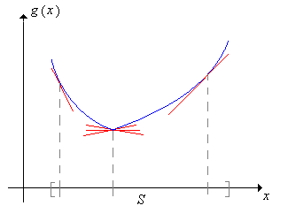
You may be more familiar with convexity in terms of the following theorem from calculus: If \(g\) has a continuous, non-negative second derivative on \(S\), then \(g\) is convex on \(S\) (since the tangent line at \(t\) is a supporting line at \(t\) for each \(t \in S\)). The next result is the single variable version of Jensen's inequality

If \(X\) takes values in an interval \(S\) and \(g: S \to \R\) is convex on \(S\), then \[ \E\left[g(X)\right] \ge g\left[\E(X)\right] \]

Proof

Note that \( \E(X) \in S \) so let \( y = a + b x \) be a supporting line for \( g \) at \( \E(X) \). Thus \(a + b \E(X) = g[\E(X)]\) and \(a + b \, X \le g(X)\). Taking expected values through the inequality gives

\[ a + b \, \E(X) = g\left[\E(X)\right] \le \E\left[g(X)\right] \]

Jensens's inequality extends easily to higher dimensions. The 2-dimensional version is particularly important, because it will be used to derive several special inequalities in the section on vector spaces of random variables. We need two definitions.

A set \(S \subseteq \R^n\) is convex if for every pair of points in \(S\), the line segment connecting those points also lies in \(S\). That is, if \(\bs x, \, \bs y \in S\) and \(p \in [0, 1]\) then \(p \bs x + (1 - p) \bs y \in S\).

Figure \(\PageIndex{2}\): A convex subset of \( \R^2 \)

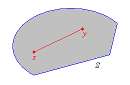
Suppose that \(S \subseteq \R^n\) is convex. A function \(g: S \to \R\) on \(S\) is convex (or concave upward) if for each \(\bs t \in S\), there exist \(a \in \R\) and \(\bs b \in \R^n\) (depending on \(\bs t\)) such that

1. \(a + \bs b \cdot \bs t = g(\bs t)\)
2. \(a + \bs b \cdot \bs x \le g(\bs x)\) for all \(\bs x \in S\)

The graph of \(\bs x \mapsto a + \bs b \cdot \bs x\) is called a supporting hyperplane for \( g \) at \(\bs t \).

In \( \R^2 \) a supporting hyperplane is an ordinary plane. From calculus, if \(g\) has continuous second derivatives on \(S\) and has a positive non-definite second derivative matrix, then \(g\) is convex on \(S\). Suppose now that \(\bs X = (X_1, X_2, \ldots, X_n)\) takes values in \(S \subseteq \R^n\), and let \(\E(\bs X ) = (\E(X_1), \E(X_2), \ldots, \E(X_n))\). The following result is the general version of Jensen's inequlaity.

If \(S\) is convex and \(g: S \to \R\) is convex on \(S\) then

\[ \E\left[g(\bs X)\right] \ge g\left[\E(\bs X)\right] \]

Proof

First \( \E(\bs X) \in S \), so let \( y = a + \bs b \cdot \bs x \) be a supporting hyperplane for \( g \) at \( \E(\bs X) \). Thus \(a + \bs b \cdot \E(\bs X) = g[\E(\bs X)]\) and \(a + \bs b \cdot \bs X \le g(\bs X)\). Taking expected values through the inequality gives \[ a + \bs b \cdot \E(\bs X ) = g\left[\E(\bs X)\right] \le \E\left[g(\bs X)\right] \]

We will study the expected value of random vectors and matrices in more detail in a later section. In both the one and \(n\)-dimensional cases, a function \(g: S \to \R\) is concave (or concave downward) if the inequality in the definition is reversed. Jensen's inequality also reverses.

Expected Value in Terms of the Quantile Function

If \( X \) has a continuous distribution with support on an interval of \( \R \), then there is a simple (but not well known) formula for the expected value of \( X \) as the integral the quantile function of \( X \). Here is the general result:

Suppose that \( X \) has a continuous distribution with support on an interval \( (a, b) \subseteq \R \). Let \( F \) denote the cumulative distribution function of \( X \) so that \( F^{-1} \) is the quantile function of \( X \). If \( g: (a, b) \to \R \) then (assuming that the expected value exists), \[ \E[g(X)] = \int_0^1 g\left[F^{-1}(p)\right] dp, \quad n \in \N \]

Proof

Suppose that \( X \) has probability density function \( f \), although the theorem is true without this assumption. Under the assumption that \( X \) has a continuous distribution with support on the interval \( (a, b) \), the distribution function \( F \) is strictly increasing on \( (a, b) \), and the quantile function \( F^{-1} \) is the ordinary inverse of \( F \). Substituting \( p = F(x) \), \( dp = F^\prime(x) \, dx = f(x) \, dx \) we have \[ \int_0^1 g\left[F^{-1}(p)\right] d p = \int_a^b g\left(F^{-1}[F(x)]\right) f(x) \, dx = \int_a^b g(x) f(x) \, dx = \E[g(X)] \]

So in particular, \( \E(X) = \int_0^1 F^{-1}(p) \, dp \).

Examples and Applications

Let \( a \in (0, \infty) \) and let \( \P(X = a) = 1 \), so that \( X \) is a constant random variable. Show that Markov's inequality is in fact equality at \( x = a \).

Solution

Of course \( \E(X) = a \). Hence \( \P(X \ge a) = 1 \) and \( \E(X) / a = 1 \).

The Exponential Distribution

Recall that the exponential distribution is a continuous distribution with probability density function \(f\) given by \[ f(t) = r e^{-r t}, \quad t \in [0, \infty) \] where \(r \in (0, \infty)\) is the rate parameter. This distribution is widely used to model failure times and other arrival times; in particular, the distribution governs the time between arrivals in the Poisson model. The exponential distribution is studied in detail in the chapter on the Poisson Process.

Suppose that \(X\) has exponential distribution with rate parameter \(r\).

1. Find \(\E(X) \) using the right distribution formula.
2. Find \( \E(X) \) using the quantile function formula.
3. Compute both sides of Markov's inequality.

Answer

1. \( \int_0^\infty e^{-r t} \, dt = \frac{1}{r} \)
2. \( \int_0^1 -\frac{1}{r} \ln(1 - p) \, dp = \frac{1}{r} \)
3. \(e^{-r t} \lt \frac{1}{r t}\) for \( t \gt 0 \)

Open the gamma experiment. Keep the default value of the stopping parameter (\( n = 1 \)), which gives the exponential distribution. Vary the rate parameter \( r \) and note the shape of the probability density function and the location of the mean. For various values of the rate parameter, run the experiment 1000 times and compare the sample mean with the distribution mean.

The Geometric Distribution

Recall that Bernoulli trials are independent trials each with two outcomes, which in the language of reliability, are called success and failure. The probability of success on each trial is \( p \in [0, 1] \). A separate chapter on Bernoulli Trials explores this random process in more detail. It is named for Jacob Bernoulli. If \( p \in (0, 1) \), the trial number \( N \) of the first success has the geometric distribution on \(\N_+\) with success parameter \(p\). The probability density function \(f\) of \( N \) is given by \[ f(n) = p (1 - p)^{n - 1}, \quad n \in \N_+ \]

Suppose that \(N\) has the geometric distribution on \( \N_+ \) with parameter \( p \in (0, 1) \).

1. Find \(\E(N)\) using the right distribution function formula.
2. Compute both sides of Markov's inequality.
3. Find \(\E(N \mid N \text{ is even })\).

Answer

1. \( \sum_{n=0}^\infty (1 - p)^n = \frac{1}{p} \)
2. \((1 - p)^{n-1} \lt \frac{1}{n p}, \quad n \in \N_+\)
3. \(\frac{2 (1 - p)^2}{p (2 - p)^2}\)

Open the negative binomial experiment. Keep the default value of the stopping parameter (\( k = 1 \)), which gives the geometric distribution. Vary the success parameter \( p \) and note the shape of the probability density function and the location of the mean. For various values of the success parameter, run the experiment 1000 times and compare the sample mean with the distribution mean.

The Pareto Distribution

Recall that the Pareto distribution is a continuous distribution with probability density function \(f\) given by \[ f(x) = \frac{a}{x^{a + 1}}, \quad x \in [1, \infty) \] where \(a \in (0, \infty)\) is a parameter. The Pareto distribution is named for Vilfredo Pareto. It is a heavy-tailed distribution that is widely used to model certain financial variables. The Pareto distribution is studied in detail in the chapter on Special Distributions.

Suppose that \(X\) has the Pareto distribution with parameter \( a \gt 1 \).

1. Find \(\E(X)\) using the right distribution function formula.
2. Find \( \E(X) \) using the quantile function formula.
3. Find \(\E(1 / X)\).
4. Show that \(x \mapsto 1 / x\) is convex on \((0, \infty)\).
5. Verify Jensen's inequality by comparing \( \E(1 / X) \) and \( 1 \big/ \E(X) \).

Answer

1. \(\int_0^1 1 \, dx + \int_1^\infty x^{-a} \, dx = \frac{a}{a - 1}\)
2. \( \int_0^1 (1 - p)^{-1/a} dp = \frac{a}{a - 1} \)
3. \(\frac{a}{a + 1}\)
4. The convexity of \( 1 / x \) is clear from the graph. Note also that \( \frac{d^2}{dx^2} \frac{1}{x} = \frac{2}{x^3} \gt 0 \) for \( x \gt 0 \).
5. \(\frac{a}{a + 1} \gt \frac{a -1}{a}\)

Open the special distribution simulator and select the Pareto distribution. Keep the default value of the scale parameter. Vary the shape parameter and note the shape of the probability density function and the location of the mean. For various values of the shape parameter, run the experiment 1000 times and compare the sample mean with the distribution mean.

A Bivariate Distribution

Suppose that \((X, Y)\) has probability density function \(f\) given by \(f(x, y) = 2 (x + y)\) for \(0 \le x \le y \le 1\).

1. Show that the domain of \(f\) is a convex set.
2. Show that \((x, y) \mapsto x^2 + y^2\) is convex on the domain of \(f\).
3. Compute \(\E\left(X^2 + Y^2\right)\).
4. Compute \(\left[\E(X)\right]^2 + \left[\E(Y)\right]^2\).
5. Verify Jensen's inequality by comparing (b) and (c).

Answer

1. Note that the domain is a triangular region.
2. The second derivative matrix is \( \left[\begin{matrix} 2 & 0 \\ 0 & 2\end{matrix}\right] \).
3. \(\frac{5}{6}\)
4. \(\frac{53}{72}\)
5. \(\frac{5}{6} \gt \frac{53}{72}\)

The Arithmetic and Geometric Means

Suppose that \(\{x_1, x_2, \ldots, x_n\}\) is a set of positive numbers. The arithmetic mean is at least as large as the geometric mean: \[ \left(\prod_{i=1}^n x_i \right)^{1/n} \le \frac{1}{n}\sum_{i=1}^n x_i \]

Proof

Let \(X\) be uniformly distributed on \(\{x_1, x_2, \ldots, x_n\}\). We apply Jensen's inequality with the natural logarithm function, which is concave on \((0, \infty)\): \[ \E\left(\ln X \right) = \frac{1}{n} \sum_{i=1}^n \ln x_i = \ln \left[ \left(\prod_{i=1}^n x_i \right)^{1/n} \right] \le \ln\left[\E(X)\right] = \ln \left(\frac{1}{n}\sum_{i=1}^n x_i \right) \] Taking exponentials of each side gives the inequality.