10.3: The Quantile Function

The Quantile Function

The quantile function for a probability distribution has many uses in both the theory and application of probability. If \(F\) is a probability distribution function, the quantile function may be used to “construct” a random variable having \(F\) as its distributions function. This fact serves as the basis of a method of simulating the “sampling” from an arbitrary distribution with the aid of a random number generator. Also, given any finite class

\(\{X_i: 1 \le i \le n\}\) of random variables, an independent class \(\{Y_i: 1 \le i \le n\}\) may be constructed, with each \(X_i\) and associated \(Y_i\) having the same (marginal) distribution. Quantile functions for simple random variables may be used to obtain an important Poisson approximation theorem (which we do not develop in this work). The quantile function is used to derive a number of useful special forms for mathematical expectation.

General concept—properties, and examples

If \(F\) is a probability distribution function, the associated quantile function \(Q\) is essentially an inverse of \(F\). The quantile function is defined on the unit interval (0, 1). For \(F\) continuous and strictly increasing at \(t\), then \(Q(u) = t\) iff \(F(t) = u\). Thus, if \(u\) is a probability value, \(t = Q(u)\) is the value of \(t\) for which \(P(X \le t) = u\).

Example 10.3.28: The Weibull distribution (3, 2, 0)

\(u = F(t) = 1 - e^{-3t^2}\) \(t \ge 0\) \(\Rightarrow\) \(t = Q(u) = \sqrt{-\text{ln } (1 - u)/3}\)

Example 10.3.29:  The Normal Distribution

The m-function norminv, based on the MATLAB function erfinv (inverse error function), calculates values of \(Q\) for the normal distribution.

The restriction to the continuous case is not essential. We consider a general definition which applies to any probability distribution function.

Definition: If \(F\) is a function having the properties of a probability distribution function, then the quantile function for \(F\) is given by

\(Q(u) = \text{inf } \{t: F(t) \ge u\}\) \(\forall u \in (0, 1)\)

We note

• If \(F(t^{*}) \ge u^{*}\), then \(t^{*} \ge \text{inf } \{t: F(t) \ge u^{*}\} = Q(u^{*})\)
• If \(F(t^{*}) < u^{*}\), then \(t^{*} < \text{inf } \{t: F(t) \ge u^{*}\} = Q(u^{*})\)

Hence, we have the important property:

(Q1) \(Q(u) \le t\) iff \(u \le F(t)\) \(\forall u \in (0, 1)\)

The property (Q1) implies the following important property:

(Q2)If \(U\)~ uniform (0, 1), then \(X = Q(U)\) has distribution function \(F_X = F\). To see this, note that \(F_X(t) = P(Q(U) \le t] = P[U \le F(t)] = F(t)\).

Property (Q2) implies that if \(F\) is any distribution function, with quantile function \(Q\), then the random variable \(X = Q(U)\), with \(U\) uniformly distributed on (0, 1), has distribution function \(F\).

Example 10.3.30:  Independent classes with prescribed distributions

Suppose \(\{X_i: 1 \le i \le n\}\) is an arbitrary class of random variables with corresponding distribution functions \(\{F_i : 1 \le i \le n\}\). Let \(\{Q_i: 1 \le i \le n\}\) be the respective quantile functions. There is always an independent class \(\{U_i: 1 \le i \le n\}\) iid uniform (0, 1) (marginals for the joint uniform distribution on the unit hypercube with sides (0, 1)). Then the random variables \(Y_i = Q_i (U_i)\), \(1 \le i \le n\), form an independent class with the same marginals as the \(X_i\).

Several other important properties of the quantile function may be established.

Figure 10.3.9. Graph of quantile function from graph of distribution function,

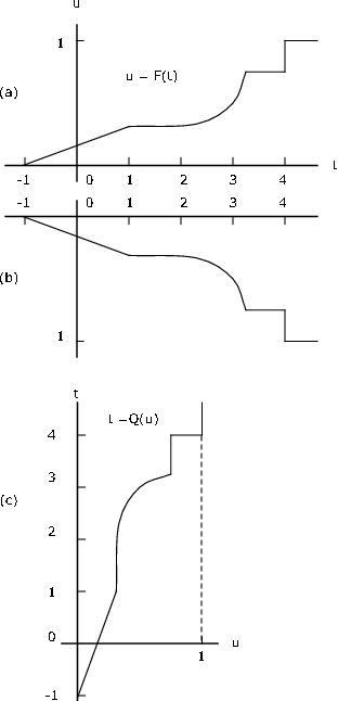
\(Q\) is left-continuous, whereas \(F\) is right-continuous.

If jumps are represented by vertical line segments, construction of the graph of \(u = Q(t)\) may be obtained by the following two step procedure:

• Invert the entire figure (including axes), then
• Rotate the resulting figure 90 degrees counterclockwise

This is illustrated in Figure 10.3.9. If jumps are represented by vertical line segments, then jumps go into flat segments and flat segments go into vertical segments.

If \(X\) is discrete with probability \(p_i\) at \(t_i\), \(1 \le i \le n\), then \(F\) has jumps in the amount \(p_i\) at each \(t_i\) and is constant between. The quantile function is a left-continuous step function having value \(t_i\) on the interval \((b_{i - 1}, b_i]\), where \(b_0 = 0\) and \(b_i = \sum_{j = 1}^{i} p_j\). This may be stated

If \(F(t_i) = b_i\), then \(Q(u) = t_i\) for \(F(t_{i - 1}) < u \le F(t_i)\)

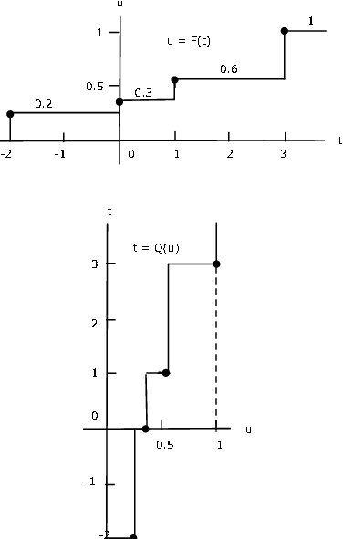
Example 10.2.31: Quantile function for a simple random variable

Suppose simple random variable \(X\) has distribution

\(X =\) [-2 0 1 3] \(PX = [0.2 0.1 0.3 0.4]

Figure 1 shows a plot of the distribution function \(F_X\). It is reflected in the horizontal axis then rotated counterclockwise to give the graph of \(Q(u\) versus \(u\).

Figure 10.3.10. Distribution and quantile functions for Example 10.3.31.

We use the analytic characterization above in developing a number of m-functions and m-procedures.

m-procedures for a simple random variable

The basis for quantile function calculations for a simple random variable is the formula above. This is implemented in the m-function dquant, which is used as an element of several simulation procedures. To plot the quantile function, we use dquanplot which employs the stairs function and plots \(X\) vs the distribution function \(FX\). The procedure dsample employs dquant to obtain a “sample” from a population with simple distribution and to calculate relative frequencies of the various values.

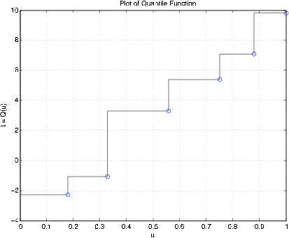
Example 10.3.32: Simple Random Variable

X =  [-2.3 -1.1 3.3 5.4 7.1 9.8];
PX = 0.01*[18 15 23 19 13 12];
dquanplot
Enter VALUES for X  X
Enter PROBABILITIES for X  PX     % See Figure 10.3.11 for plot of results
rand('seed',0)                 % Reset random number generator for reference
dsample
Enter row matrix of values  X
Enter row matrix of probabilities  PX
Sample size n  10000

    Value      Prob    Rel freq
   -2.3000    0.1800    0.1805
   -1.1000    0.1500    0.1466
    3.3000    0.2300    0.2320
    5.4000    0.1900    0.1875
    7.1000    0.1300    0.1333
    9.8000    0.1200    0.1201
Sample average ex = 3.325
Population mean E[X] = 3.305
Sample variance = 16.32
Population variance Var[X] = 16.33

Figure 10.3.11. Quantile function for Example 10.3.32.

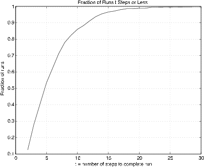
Sometimes it is desirable to know how many trials are required to reach a certain value, or one of a set of values. A pair of m-procedures are available for simulation of that problem. The first is called targetset. It calls for the population distribution and then for the designation of a “target set” of possible values. The second procedure, targetrun, calls for the number of repetitions of the experiment, and asks for the number of members of the target set to be reached. After the runs are made, various statistics on the runs are calculated and displayed.

Example 10.3.33

X = [-1.3 0.2 3.7 5.5 7.3];     % Population values
PX = [0.2 0.1 0.3 0.3 0.1];     % Population probabilities
E = [-1.3 3.7];                 % Set of target states
targetset
Enter population VALUES  X
Enter population PROBABILITIES  PX
The set of population values is
   -1.3000    0.2000    3.7000    5.5000    7.3000
Enter the set of target values  E
Call for targetrun

rand('seed',0)                  % Seed set for possible comparison
targetrun
Enter the number of repetitions  1000
The target set is
   -1.3000    3.7000
Enter the number of target values to visit  2
The average completion time is 6.32
The standard deviation is 4.089
The minimum completion time is 2
The maximum completion time is 30
To view a detailed count, call for D.
The first column shows the various completion times;
the second column shows the numbers of trials yielding those times
% Figure 10.6.4 shows the fraction of runs requiring t steps or less

Figure 10.3.12. Fraction of runs requiring \(t\) steps or less.

m-procedures for distribution functions

A procedure dfsetup utilizes the distribution function to set up an approximate simple distribution. The m-procedure quanplot is used to plot the quantile function. This procedure is essentially the same as dquanplot, except the ordinary plot function is used in the continuous case whereas the plotting function stairs is used in the discrete case. The m-procedure qsample is used to obtain a sample from the population. Since there are so many possible values, these are not displayed as in the discrete case.

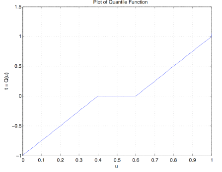
Example 10.3.34: Quantile function associated with a distribution function

F = '0.4*(t + 1).*(t < 0) + (0.6 + 0.4*t).*(t >= 0)';  % String
dfsetup
Distribution function F is entered as a string
variable, either defined previously or upon call
Enter matrix [a b] of X-range endpoints  [-1 1]
Enter number of X approximation points  1000
Enter distribution function F as function of t  F
Distribution is in row matrices X and PX
quanplot
Enter row matrix of values  X
Enter row matrix of probabilities  PX
Probability increment h  0.01          % See Figure 10.3.13 for plot
qsample
Enter row matrix of X values  X
Enter row matrix of X probabilities  PX
Sample size n  1000
Sample average ex = -0.004146
Approximate population mean E(X) = -0.0004002     % Theoretical = 0
Sample variance vx = 0.25
Approximate population variance V(X) = 0.2664

Figure 10.3.13. Quantile function for Example 10.3.34.

 

m-procedures for density functions

An m- procedure acsetup is used to obtain the simple approximate distribution. This is essentially the same as the procedure tuappr, except that the density function is entered as a string variable. Then the procedures quanplot and qsample are used as in the case of distribution functions.

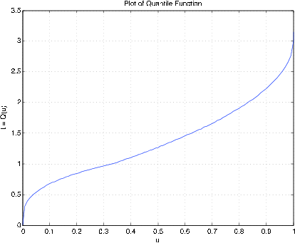
Example 10.3.35:  Quantile function associated with a density function

acsetup
Density f is entered as a string variable.
either defined previously or upon call.
Enter matrix [a b] of x-range endpoints  [0 3]
Enter number of x approximation points  1000
Enter density as a function of t  '(t.^2).*(t<1) + (1- t/3).*(1<=t)'
Distribution is in row matrices X and PX
quanplot
Enter row matrix of values  X
Enter row matrix of probabilities  PX
Probability increment h  0.01               % See Figure 10.3.14 for plot
rand('seed',0)
qsample
Enter row matrix of values  X
Enter row matrix of probabilities  PX
Sample size n  1000
Sample average ex = 1.352
Approximate population mean E(X) = 1.361  % Theoretical = 49/36 = 1.3622
Sample variance vx = 0.3242
Approximate population variance V(X) = 0.3474    % Theoretical = 0.3474

Figure 10.3.14. Quantile function for Example 10.3.35.