
10.2: Function of Random Vectors
- Page ID
- 10877

Introduction
The general mapping approach for a single random variable and the discrete alternative extends to functions of more than one variable. It is convenient to consider the case of two random variables, considered jointly. Extensions to more than two random variables are made similarly, although the details are more complicated.
The general approach extended to a pair
Consider a pair \(\{X, Y\}\) having joint distribution on the plane. The approach is analogous to that for a single random variable with distribution on the line.
To find \(P((X, Y) \in Q)\).
- Mapping approach. Simply find the amount of probability mass mapped into the set \(Q\) on the plane by the random vector \(W = (X, Y)\).
- In the absolutely continuous case, calculate \(\int \int_Q f_{XY}\).
- In the discrete case, identify those vector values \((t_i, u_j)\) of \((X, Y)\) which are in the set \(Q\) and add the associated probabilities.
- Discrete alternative. Consider each vector value \((t_i, u_j)\) of \((X, Y)\). Select those which meet the defining conditions for \(Q\) and add the associated probabilities. This is the approach we use in the MATLAB calculations. It does not require that we describe geometrically the region \(Q\).
To find \(P(g(X,Y) \in M)\). \(g\) is real valued and \(M\) is a subset the real line.
- Mapping approach. Determine the set \(Q\) of all those \((t, u)\) which are mapped into \(M\) by the function \(g\). Now
\(W(\omega) = (X(\omega), Y(\omega)) \in Q\) iff \(g((X(\omega), Y(\omega)) \in M\) Hence
\(\{\omega: g(X(\omega), Y(\omega)) \in M\} = \{\omega: (X(\omega), Y(\omega)) \in Q\}\)
Since these are the same event, they must have the same probability. Once \(Q\) is identified on the plane, determine \(P((X, Y) \in Q)\) in the usual manner (see part a, above).
- Discrete alternative. For each possible vector value \((t_i, u_j)\) of \((X, Y)\), determine whether \(g(t_i, u_j)\) meets the defining condition for \(M\). Select those \((t_i, u_j)\) which do and add the associated probabilities.
We illustrate the mapping approach in the absolutely continuous case. A key element in the approach is finding the set \(Q\) on the plane such that \(g(X, Y) \in M\) iff \((X, Y) \in Q\). The desired probability is obtained by integrating \(f_{XY}\) over \(Q\).
Example 10.2.15. A numerical example
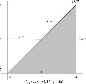
The pair \(\{X, Y\}\) has joint density \(f_{XY} (t, u) = \dfrac{6}{37} (t + 2u)\) on the region bounded by \(t = 0\), \(t = 2\), \(u = 0\), \(u = \text{max} \{1, t\}\) (see Figure 1). Determine \(P(Y \le X) = P(X - Y \ge 0)\). Here \(g(t, u) = t - u\) and \(M = [0, \infty)\). Now \(Q = \{(t, u) : t - u \ge 0\} = \{(t, u) : u \le t \}\) which is the region on the plane on or below the line \(u = t\). Examination of the figure shows that for this region, \(f_{XY}\) is different from zero on the triangle bounded by \(t = 2\), \(u = 0\), and \(u = t\). The desired probability is
\(P(Y \le X) = \int_{0}^{2} \int_{0}^{t} \dfrac{6}{37} (t + 2u) du\ dt = 32/37 \approx 0.8649\)
Example 10.2.16. The density for the sum X+Y
Suppose the pair \(\{X, Y\}\) has joint density \(f_{XY}\). Determine the density for
\(Z = X + Y\)
Solution
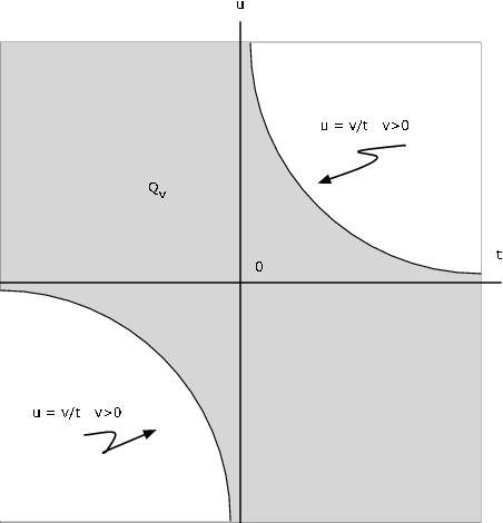
\(F_Z (v) = P(X + Y \le v) = P((X, Y) \in Q_v)\) where \(Q_v = \{(t, u) : t + u \le v\} = \{(t, u): u \le v - t\}\)
For any fixed \(v\), the region \(Q_v\) is the portion of the plane on or below the line \(u = v - t\) (see Figure 10.2.2). Thus
\(F_Z (v) = \int \int_{Q} f_{XY} = \int_{-\infty}^{\infty} \int_{-\infty}^{v - t} f_{XY} (t, u) du\ dt\)
Differentiating with the aid of the fundamental theorem of calculus, we get
\(f_Z (v) = \int_{\infty}^{\infty} f_{XY} (t, v - t)\ dt\)
This integral expresssion is known as a convolution integral.
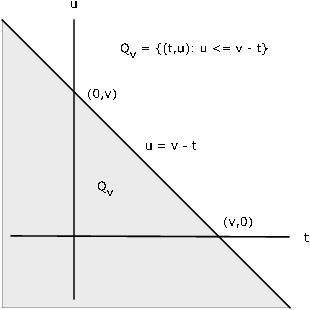
Figure 10.2.2. Region \(Q_v\) for \(X + Y \le v\).
Example 10.2.17. Sum of joint uniform random variables
Suppose the pair \(\{X, Y\}\) has joint uniform density on the unit square \(0 \le t \le 1, 0 \le u \le 1\).. Determine the density for \(Z = X + Y\).
Solution
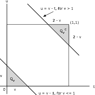
\(F_Z (v)\) is the probability in the region \(Q_v: u \le v - t\). Now \(P_{XY} (Q_v) = 1 - P_{XY} (Q_{v}^{c})\), where the complementary set \(Q_{v}^{c}\) is the set of points above the line. As Figure 3 shows, for \(v \le 1\), the part of \(Q_v\) which has probability mass is the lower shaded triangular region on the figure, which has area (and hence probability) \(v^2\)/2. For \(v\) > 1, the complementary region \(Q_{v}^{c}\) is the upper shaded region. It has area \((2 - v)^2/2\). so that in this case, \(P_{XY} (Q_v) = 1 - (2 - v)^2/2\). Thus,
\(F_Z (v) = \dfrac{v^2}{2}\) for \(0 \le v \le 1\) and \(F_Z (v) = 1 - \dfrac{(2 - v)^2}{2}\) for \(1 \le v \le 2\)
Differentiation shows that \(Z\) has the symmetric triangular distribution on [0, 2], since
\(f_Z (v) = v\) for \(0 \le v \le 1\) and \(f_Z(v) = (2 - v)\) for \(1 \le v \le 2\)
With the use of indicator functions, these may be combined into a single expression
\(f_Z (v) = I_{[0, 1]} (v) v + I_{(1, 2]} (2 - v)\)
ALTERNATE Solution
Since \(f_{XY} (t, u) = I_{[0, 1]} (t) I_{[0, 1]} (u)\), we have \(f_{XY} (t, v - t) = I_{[0, 1]} (t) I_{[0, 1]} (v - t)\). Now \(0 \le v - t \le 1\) iff \(v - 1 \le t \le v\), so that
\(f_{XY} (t, v - t) = I_{[0, 1]} (v) I_{[0, v]} (t) + I_{(1, 2]} (v) I_{[v - 1, 1]} (t)\)
Integration with respect to \(t\) gives the result above.
Independence of functions of independent random variables
Suppose \(\{X, Y\}\) is an independent pair. Let \(Z = g(X), W = h(Y)\). Since
\(Z^{-1} (M) = X^{-1} [g^{-1} (M)]\) and \(W^{-1} (N) = Y^{-1} [h^{-1} (N)]\)
the pair \(\{Z^{-1} (M), W^{-1} (N)\}\) is independent for each pair \(\{M, N\}\). Thus, the pair \(\{Z, W\}\) is independent.
If \(\{X, Y\}\) is an independent pair and \(Z = g(X)\), \(W = g(X)\), then the pair \(\{Z, W\}\) is independent. However, if \(Z = g(X, Y)\) and \(W = h(X, Y)\), then in general \(\{Z, W\}\) is not independent. This is illustrated for simple random variables with the aid of the m-procedure jointzw at the end of the next section.
Example 10.2.18. Independence of simple approximations to an independent pair
Suppose \(\{X, Y\}\) is an independent pair with simple approximations \(X_s\) and \(Y_s\) as described in Distribution Approximations.
\(X_s = \sum_{i = 1}^{n} t_i I_{E_i} = \sum_{i = 1}^{n} t_i I_{M_i} (X)\) and \(Y_s = \sum_{j = 1}^{m} u_j I_{F_j} = \sum_{j = 1}^{m} u_j I_{N_j} (Y)\)
As functions of \(X\) and \(Y\), respectively, the pair \(\{X_s, Y_s\}\) is independent. Also each pair \(\{I_{M_i}(X), I_{N_j} (Y)\}\) is independent.
Use of MATLAB on pairs of simple random variables
In the single-variable case, we use array operations on the values of \(X\) to determine a matrix of values of \(g(X)\). In the two-variable case, we must use array operations on the calculating matrices \(t\) and \(u\) to obtain a matrix \(G\) whose elements are \(g(t_i, u_j)\). To obtain the distribution for \(Z = g(X, Y)\), we may use the m-function csort on \(G\) and the joint probability matrix \(P\). A first step, then, is the use of jcalc or icalc to set up the joint distribution and the calculating matrices. This is illustrated in the following example.
Example 10.2.19.
% file jdemo3.m
% data for joint simple distribution
X = [-4 -2 0 1 3];
Y = [0 1 2 4];
P = [0.0132    0.0198    0.0297    0.0209    0.0264;
     0.0372    0.0558    0.0837    0.0589    0.0744;
     0.0516    0.0774    0.1161    0.0817    0.1032;
     0.0180    0.0270    0.0405    0.0285    0.0360];
jdemo3                % Call for data
jcalc                 % Set up of calculating matrices t, u.
Enter JOINT PROBABILITIES (as on the plane)  P
Enter row matrix of VALUES of X  X
Enter row matrix of VALUES of Y  Y
 Use array operations on matrices X, Y, PX, PY, t, u, and P
G = t.^2 -3*u;        % Formation of G = [g(ti,uj)]
M = G >= 1;           % Calculation using the XY distribution
PM = total(M.*P)      % Alternately, use total((G>=1).*P)
PM =  0.4665
[Z,PZ] = csort(G,P);
PM = (Z>=1)*PZ'     % Calculation using the Z distribution
PM =  0.4665
disp([Z;PZ]')         % Display of the Z distribution
  -12.0000    0.0297
  -11.0000    0.0209
   -8.0000    0.0198
   -6.0000    0.0837
   -5.0000    0.0589
   -3.0000    0.1425
   -2.0000    0.1375
         0    0.0405
    1.0000    0.1059
    3.0000    0.0744
    4.0000    0.0402
    6.0000    0.1032
    9.0000    0.0360
   10.0000    0.0372
   13.0000    0.0516
   16.0000    0.0180
We extend the example above by considering a function \(W = h(X, Y)\) which has a composite definition.
Example 10.2.20. Continuation of example 10.2.19
Let
\(W = \begin{cases} X & \text{ for } X + Y \ge 1 \\ X^2 + Y^2 & \text{ for } X + Y < 1 \end{cases}\) Determine the distribution for \(W\)
H = t.*(t+u>=1) + (t.^2 + u.^2).*(t+u<1);  % Specification of h(t,u)


[W,PW] = csort(H,P);                       % Distribution for W = h(X,Y)
disp([W;PW]')
   -2.0000    0.0198
         0    0.2700
    1.0000    0.1900
    3.0000    0.2400
    4.0000    0.0270
    5.0000    0.0774
    8.0000    0.0558
   16.0000    0.0180
   17.0000    0.0516
   20.0000    0.0372
   32.0000    0.0132
ddbn                                        % Plot of distribution function
Enter row matrix of values  W
Enter row matrix of probabilities  PW
print                                       % See Figure 10.2.4
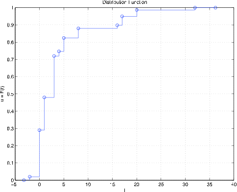
Figure 10.2.4. Distribution for random variable \(W\) in Example 10.2.20.
Joint distributions for two functions of \((X, Y)\)
In previous treatments, we use csort to obtain the marginal distribution for a single function \(Z = g(X, Y)\). It is often desirable to have the joint distribution for a pair \(Z = g(X, Y)\) and \(W = h(X, Y)\). As special cases, we may have \(Z = X\) or \(W = Y\). Suppose
\(Z\) has values [\(z_1\) \(z_2\) \(\cdot\cdot\cdot\) \(z_c\)] and \(W\) has calues [\(w_1\) \(w_2\) \(\cdot\cdot\cdot\) \(w_c\)]
The joint distribution requires the probability of each pair, \(P(W = w_i, Z = z_j)\). Each such pair of values corresponds to a set of pairs of \(X\) and \(Y\) values. To determine the joint probability matrix \(PZW\) for \((Z, W)\) arranged as on the plane, we assign to each position \((i, j)\) the probability \(P(W = w_i, Z=z_j)\), with values of \(W\) increasing upward. Each pair of (\(W, Z\)) values corresponds to one or more pairs of (\(Y, X\)) values. If we select and add the probabilities corresponding to the latter pairs, we have \(P(W = w_i, Z = z_j)\). This may be accomplished as follows:
Set up calculation matrices \(t\) and \(u\) as with jcalc.
Use array arithmetic to determine the matrices of values \(G = [g(t, u)]\) and \(H = [h(t, u)]\).
Use csort to determine the \(Z\) and \(W\) value matrices and the \(PZ\) and \(PW\) marginal probability matrices.
For each pair \((w_i, z_j)\), use the MATLAB function find to determine the positions a for which
Assign to the (\(i, j\)) position in the joint probability matrix \(PZW\) for (\(Z, W\)) the probability
We first examine the basic calculations, which are then implemented in the m-procedure jointzw.
Example 10.2.21. Illustration of the basic joint calculations
% file jdemo7.m
P = [0.061  0.030  0.060  0.027  0.009;
       0.015  0.001  0.048  0.058  0.013;
       0.040  0.054  0.012  0.004  0.013;
       0.032  0.029  0.026  0.023  0.039;
       0.058  0.040  0.061  0.053  0.018;
       0.050  0.052  0.060  0.001  0.013];
X = -2:2;
Y = -2:3;
jdemo7                      % Call for data in jdemo7.m
jcalc                       % Used to set up calculation matrices t, u
- - - - - - - - - -
H = u.^2                    % Matrix of values for W = h(X,Y)
H =
     9     9     9     9     9
     4     4     4     4     4
     1     1     1     1     1
     0     0     0     0     0
     1     1     1     1     1
     4     4     4     4     4
G = abs(t)                  % Matrix of values for Z = g(X,Y)

G =
     2     1     0     1     2
     2     1     0     1     2
     2     1     0     1     2
     2     1     0     1     2
     2     1     0     1     2
     2     1     0     1     2
[W,PW] = csort(H,P)         % Determination of marginal for W
W =     0     1     4     9
PW =    0.1490    0.3530    0.3110    0.1870
[Z,PZ] = csort(G,P)         % Determination of marginal for Z
Z =     0     1     2
PZ =    0.2670    0.3720    0.3610
r = W(3)                    % Third value for W
r =   4
s = Z(2)                    % Second value for Z
s =   1
To determine \(P(W = 4, Z = 1)\), we need to determine the (\(t, u\)) positions for which this pair of (\(W, Z\)) values is taken on. By inspection, we find these to be (2,2), (6,2), (2,4), and (6,4). Then \(P(W = 4, Z = 1)\) is the total probability at these positions. This is 0.001 + 0.052 + 0.058 + 0.001 = 0.112. We put this probability in the joint probability matrix \(PZW\) at the \(W = 4, Z = 1\) position. This may be achieved by MATLAB with the following operations.
[i,j] = find((H==W(3))&(G==Z(2)));  % Location of (t,u) positions
disp([i j])                         % Optional display of positions
     2     2
     6     2
     2     4
     6     4
a = find((H==W(3))&(G==Z(2)));      % Location in more convenient form
P0 = zeros(size(P));                % Setup of zero matrix
P0(a) = P(a)                        % Display of designated probabilities in P
P0 =
         0         0         0         0         0
         0    0.0010         0    0.0580         0
         0         0         0         0         0
         0         0         0         0         0
         0         0         0         0         0
         0    0.0520         0    0.0010         0
PZW = zeros(length(W),length(Z))    % Initialization of PZW matrix
PZW(3,2) = total(P(a))              % Assignment to PZW matrix with
PZW =    0         0         0      % W increasing downward
         0         0         0
         0    0.1120         0
         0         0         0
PZW = flipud(PZW)                   % Assignment with W increasing upward
PZW =
         0         0         0
         0    0.1120         0
         0         0         0
         0         0         0
The procedure jointzw carries out this operation for each possible pair of \(W\) and \(Z\) values (with the flipud operation coming only after all individual assignments are made).
example 10.2.22. joint distribution for z = g(x,y) = ||x| - y| and w = h(x, y) = |xy|
% file jdemo3.m   data for joint simple distribution
X = [-4 -2 0 1 3];
Y = [0 1 2 4];
P = [0.0132    0.0198    0.0297    0.0209    0.0264;
     0.0372    0.0558    0.0837    0.0589    0.0744;
     0.0516    0.0774    0.1161    0.0817    0.1032;
     0.0180    0.0270    0.0405    0.0285    0.0360];
jdemo3          % Call for data
jointzw         % Call for m-program
Enter joint prob for (X,Y): P
Enter values for X: X
Enter values for Y: Y
Enter expression for g(t,u): abs(abs(t)-u)
Enter expression for h(t,u): abs(t.*u)
Use array operations on Z, W, PZ, PW, v, w, PZW
disp(PZW)
    0.0132         0         0         0         0
         0    0.0264         0         0         0
         0         0    0.0570         0         0
         0    0.0744         0         0         0
    0.0558         0         0    0.0725         0
         0         0    0.1032         0         0
         0    0.1363         0         0         0
    0.0817         0         0         0         0
    0.0405    0.1446    0.1107    0.0360    0.0477
EZ = total(v.*PZW)
EZ =   1.4398

ez = Z*PZ'       % Alternate, using marginal dbn
ez =   1.4398
EW = total(w.*PZW)
EW =   2.6075
ew = W*PW'       % Alternate, using marginal dbn
ew =   2.6075
M = v > w;           % P(Z>W)
PM = total(M.*PZW)
PM =   0.3390
At noted in the previous section, if \(\{X, Y\}\) is an independent pair and \(Z = g(X)\),
\(W = h(Y)\), then the pair {\(Z, W\)} is independent. However, if \(Z = g(X, Y)\) and
\(W = h(X, Y)\), then in general the pair {\(Z, W\)} is not independent. We may illustrate this with the aid of the m-procedure jointzw
Example 10.2.23. Functions of independent random variables
jdemo3
itest
Enter matrix of joint probabilities  P
The pair {X,Y} is independent           % The pair {X,Y} is independent
jointzw
Enter joint prob for (X,Y): P
Enter values for X: X
Enter values for Y: Y
Enter expression for g(t,u): t.^2 - 3*t  % Z = g(X)
Enter expression for h(t,u): abs(u) + 3  % W = h(Y)
Use array operations on Z, W, PZ, PW, v, w, PZW
itest
Enter matrix of joint probabilities  PZW
The pair {X,Y} is independent           % The pair {g(X),h(Y)} is independent
jdemo3                                  % Refresh data
jointzw
Enter joint prob for (X,Y): P
Enter values for X: X
Enter values for Y: Y
Enter expression for g(t,u): t+u         % Z = g(X,Y)
Enter expression for h(t,u): t.*u        % W = h(X,Y)
Use array operations on Z, W, PZ, PW, v, w, PZW
itest
Enter matrix of joint probabilities  PZW
The pair {X,Y} is NOT independent  % The pair {g(X,Y),h(X,Y)} is not indep
To see where the product rule fails, call for D  % Fails for all pairs
Absolutely continuous case: analysis and approximation
As in the analysis Joint Distributions, we may set up a simple approximation to the joint distribution and proceed as for simple random variables. In this section, we solve several examples analytically, then obtain simple approximations.
Example 10.2.24. Distribution for a product
Suppose the pair \(\{X, Y\}\) has joint density \(f_{XY}\). Let \(Z = XY\). Determine \(Q_v\) such that \(P(Z \le v) = P((X, Y) \in Q_v)\).
Solution
\(Q_v = \{(t, u) : tu \le v\} = \{(t, u): t > 0, u \le v/t\} \bigvee \{(t, u) : t < 0, u \ge v/t\}\}\)
Example 10.2.25.
\(\{X, Y\}\) ~ uniform on unit square
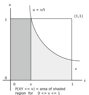
\(f_{XY} (t, u) = 1\). Then (see Figure 10.2.6)
\(P(XY \le v) = \int \int_{Q_v} 1 du\ dt\) where \(Q_v = \{(t, u): 0 \le t \le 1, 0 \le u \le \text{min } \{1, v/t\}\}\)
Integration shows
\(F_Z (v) = P(XY \le v) = v(1 - \text{ln } (v))\) so that \(f_Z (v) = - \text{ln } (v) = \text{ln } (1/v)\), \(0 < v \le 1\)
For \(v = 0.5\), \(F_Z (0.5) = 0.8466\).
% Note that although f = 1, it must be expressed in terms of t, u.
tuappr
Enter matrix [a b] of X-range endpoints  [0 1]
Enter matrix [c d] of Y-range endpoints  [0 1]
Enter number of X approximation points  200
Enter number of Y approximation points  200
Enter expression for joint density  (u>=0)&(t>=0)
Use array operations on X, Y, PX, PY, t, u, and P
G = t.*u;
[Z,PZ] = csort(G,P);
p = (Z<=0.5)*PZ'
p =  0.8465                 % Theoretical value 0.8466, above
Example 10.2.26. Continuation of example 5 from "Random Vectors and Joint Distributions"
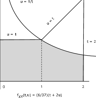
The pair \(\{X, Y\}\) has joint density \(f_{XY} (t, u) = \dfrac{6}{37} (t + 2u)\) on the region bounded by \(t = 0\), \(t = 2\) and \(u = \text{max } \{1, t\}\)(see Figure 7). Let \(Z = XY\). Determine \(P(Z \le 1)\).
Analytic Solution
Reference to Figure 10.2.7 shows that
\(P((X, Y) \in Q = \dfrac{6}{37} \int_{0}^{1} \int_{0}^{1} (t + 2u) du\ dt + \dfrac{6}{37} \int_{1}^{2} \int_{0}^{1/t} (t + 2u) du\ dt = 9/37 + 9/37 = 18/37 \approx 0.4865\)
APPROXIMATE Solution
tuappr
Enter matrix [a b] of X-range endpoints  [0 2]
Enter matrix [c d] of Y-range endpoints  [0 2]
Enter number of X approximation points  300
Enter number of Y approximation points  300
Enter expression for joint density  (6/37)*(t + 2*u).*(u<=max(t,1))
Use array operations on X, Y, PX, PY, t, u, and P
Q = t.*u<=1;
PQ = total(Q.*P)
PQ =  0.4853             % Theoretical value 0.4865, above
G = t.*u;                % Alternate, using the distribution for Z
[Z,PZ] = csort(G,P);
PZ1 = (Z<=1)*PZ'
PZ1 = 0.4853
In the following example, the function \(g\) has a compound definition. That is, it has a different rule for different parts of the plane.
Example 10.2.27. A compound function
The pair \(\{X, Y\}\) has joint density \(f_{XY} (t, u) = \dfrac{2}{3} (t + 2u)\) on the unit square \(0 \le t \le 1\), \(0 \le u \le 1\).
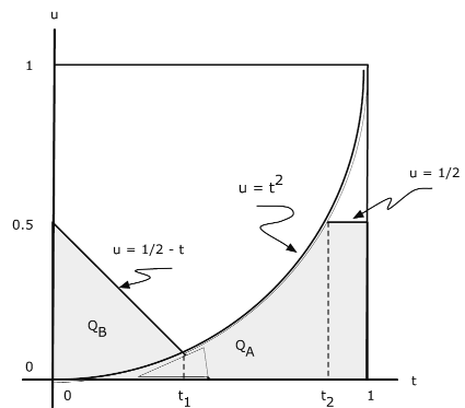
\(Z = \begin{cases} X & \text{for } X^2 - Y \ge 0 \\ X + Y & \text{for } X^2 - Y < 0 \end{cases} = I_Q (X, Y) Y + I_{Q^c} (X, Y) (X + Y)\)
for \(Q = \{(t, u): u \le t^2\}\). Determine \(P(Z <= 0.5)\).
Analytical Solution
\(P(Z \le 1/2) = P(Y \le 1/2, Y \le X^2) + P(X + Y \le 1/2, Y > X^2) = P((X, Y) \in Q_A \bigvee Q_B)\)
where \(Q_A = \{(t, u) : u \le 1/2, u \le t^2\}\) and \(Q_B = \{(t, u): t + u \le 1/2, u > t^2\}\). Reference to Figure 10.2.8 shows that this is the part of the unit square for which \(u \le \text{min } (\text{max } (1/2 - t, t^2), 1/2)\). We may break up the integral into three parts. Let \(1/2 - t_1 = t_1^2\) and \(t_2^2 = 1/2\). Then
\(P(Z \le 1/2) = \dfrac{2}{3} \int_{0}^{t_1} \int_{0}^{1/2 - t} (t + 2u) du\ dt + \dfrac{2}{3} \int_{t_1}^{t_2} \int_{0}^{t^2} (t + 2u) du\ dt + \dfrac{2}{3} \int_{t_2}^{1} \int_{0}^{1/2} (t + 2u) du \ dt = 0.2322\)
APPROXIMATE Solution
tuappr
Enter matrix [a b] of X-range endpoints  [0 1]
Enter matrix [c d] of Y-range endpoints  [0 1]
Enter number of X approximation points  200
Enter number of Y approximation points  200
Enter expression for joint density  (2/3)*(t + 2*u)
Use array operations on X, Y, PX, PY, t, u, and P
Q = u <= t.^2;
G = u.*Q + (t + u).*(1-Q);
prob = total((G<=1/2).*P)
prob =  0.2328          % Theoretical is 0.2322, above
The setup of the integrals involves careful attention to the geometry of the system. Once set up, the evaluation is elementary but tedious. On the other hand, the approximation proceeds in a straightforward manner from the normal description of the problem. The numerical result compares quite closely with the theoretical value and accuracy could be improved by taking more subdivision points.