6.6: Randomization Test (Special Topic)
- Page ID
- 290
Cardiopulmonary resuscitation (CPR) is a procedure commonly used on individuals suffering a heart attack when other emergency resources are not available. This procedure is helpful in maintaining some blood circulation, but the chest compressions involved can also cause internal injuries. Internal bleeding and other injuries complicate additional treatment efforts following arrival at a hospital. For instance, blood thinners may be used to help release a clot that is causing the heart attack. However, the blood thinner would negatively affect an internal injury. Here we consider an experiment for patients who underwent CPR for a heart attack and were subsequently admitted to a hospital.( Efficacy and safety of thrombolytic therapy after initially unsuccessful cardiopulmonary resuscitation: a prospective clinical trial, by Bottiger et al., The Lancet, 2001.) These patients were randomly divided into a treatment group where they received a blood thinner or the control group where they did not receive the blood thinner. The outcome variable of interest was whether the patients survived for at least 24 hours.
Example \(\PageIndex{1}\)
Form hypotheses for this study in plain and statistical language. Let \(p_c\) represent the true survival proportion in the control group and \(p_t\) represent the survival proportion for the treatment group.
Solution
We are interested in whether the blood thinners are helpful or harmful, so this should be a two-sided test.
- H0: Blood thinners do not have an overall survival effect, i.e. the survival proportions are the same in each group. \[p_t - p_c = 0.\]
- HA: Blood thinners do have an impact on survival. \[p_t - p_c \ne 0.\]
Large Sample Framework for a Difference in Two Proportions
There were 50 patients in the experiment who did not receive the blood thinner and 40 patients who did. The study results are shown in Table 6.22.
| Survived | Died | Total | |
|---|---|---|---|
|
Control Treatment |
11 14 |
39 26 |
50 40 |
| Total | 25 | 65 | 90 |
Exercise \(\PageIndex{1}\)
What is the observed survival rate in the control group? And in the treatment group? Also, provide a point estimate of the difference in survival proportions of the two groups: \(\hat {p}_t - \hat {p}_c\).
Solution
Observed control survival rate:
\[p_c = \dfrac {11}{50} = 0.22.\]
Treatment survival rate:
\[p_t = \dfrac {14}{40} = 0.35.\]
Observed difference:
\[\hat {p}_t - \hat {p}_c = 0.35 - 0.22 = 0.13.\]
According to the point estimate, there is a 13% increase in the survival proportion when patients who have undergone CPR outside of the hospital are treated with blood thinners. However, we wonder if this difference could be due to chance. We'd like to investigate this using a large sample framework, but we first need to check the conditions for such an approach.
Example \(\PageIndex{2}\)
Can the point estimate of the difference in survival proportions be adequately modeled using a normal distribution?
Solution
We will assume the patients are independent, which is probably reasonable. The success-failure condition is also satisfied. Since the proportions are equal under the null, we can compute the pooled proportion,
\[\hat {p} = \dfrac {(11 + 14)}{(50 + 40)} = 0.278,\]
for checking conditions. We nd the expected number of successes (13.9, 11.1) and failures (36.1, 28.9) are above 10. The normal model is reasonable.
While we can apply a normal framework as an approximation to nd a p-value, we might keep in mind that the expected number of successes is only 13.9 in one group and 11.1 in the other. Below we conduct an analysis relying on the large sample normal theory. We will follow up with a small sample analysis and compare the results.
Example \(\PageIndex{3}\)
Assess the hypotheses presented in Example 6.53 using a large sample framework. Use a significance level of \(\alpha = 0.05\).
Solution
We suppose the null distribution of the sample difference follows a normal distribution with mean 0 (the null value) and a standard deviation equal to the standard error of the estimate. The null hypothesis in this case would be that the two proportions are the same, so we compute the standard error using the pooled standard error formula from Equation (6.16) on page 273:
\[SE = \sqrt {\dfrac {p(1 - p)}{n_t} + \dfrac {p(1 - p)}{n_c}} \approx \sqrt {\dfrac {0.278(1 - 0.278)}{40} + \dfrac {0.278(1 - 0.278)}{50}} = 0.095\]
where we have used the pooled estimate \(( \hat {p} = \dfrac {11+14}{50+40} = 0.278)\) in place of the true proportion, p.
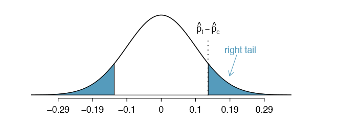
The null distribution with mean zero and standard deviation 0.095 is shown in Figure 6.23. We compute the tail areas to identify the p-value. To do so, we use the Z score of the point estimate:
\[Z = \dfrac {(\hat {p}_t - \hat {p}_c) - \text {null value}}{SE} = \dfrac {0.13 - 0}{0.095} = 1.37\]
If we look this Z score up in Appendix B.1, we see that the right tail has area 0.0853. The p-value is twice the single tail area: 0.176. This p-value does not provide convincing evidence that the blood thinner helps. Thus, there is insufficient evidence to conclude whether or not the blood thinner helps or hurts. (Remember, we never "accept" the null hypothesis - we can only reject or fail to reject.)

The p-value 0.176 relies on the normal approximation. We know that when the samples sizes are large, this approximation is quite good. However, when the sample sizes are relatively small as in this example, the approximation may only be adequate. Next we develop a simulation technique, apply it to these data, and compare our results. In general, the small sample method we develop may be used for any size sample, small or large, and should be considered as more accurate than the corresponding large sample technique.
Simulating a Difference under the null Distribution
The ideas in this section were first introduced in the optional Section 1.8. Suppose the null hypothesis is true. Then the blood thinner has no impact on survival and the 13% difference was due to chance. In this case, we can simulate null differences that are due to chance using a randomization technique. (The test procedure we employ in this section is formally called a permutation test). By randomly assigning "fake treatment" and "fake control" stickers to the patients' files, we could get a new grouping - one that is completely due to chance. The expected difference between the two proportions under this simulation is zero.
We run this simulation by taking 40 treatment fake and 50 control fake labels and randomly assigning them to the patients. The label counts of 40 and 50 correspond to the number of treatment and control assignments in the actual study. We use a computer program to randomly assign these labels to the patients, and we organize the simulation results into Table 6.24.
| Survived | Died | Total | |
|---|---|---|---|
|
Control_fake |
15 |
35 |
50 |
| Treatment_fake | 10 | 30 | 40 |
| Total | 25 | 65 | 90 |
Exercise \(\PageIndex{2}\)
What is the difference in survival rates between the two fake groups in Table 6.24? How does this compare to the observed 13% in the real groups?
Solution
The difference is \(\hat {p}_{\text {t;fake}} - \hat {p}_{\text {c;fake}} = \dfrac {10}{40} - \dfrac {15}{50} = -0.05\), which is closer to the null value p0 = 0 than what we observed.
The difference computed in Exercise 6.57 represents a draw from the null distribution of the sample differences. Next we generate many more simulated experiments to build up the null distribution, much like we did in Section 6.5.2 to build a null distribution for a one sample proportion.
Caution: Simulation in the two proportion case requires that the null difference is zero
The technique described here to simulate a difference from the null distribution relies on an important condition in the null hypothesis: there is no connection between the two variables considered. In some special cases, the null difference might not be zero, and more advanced methods (or a large sample approximation, if appropriate) would be necessary.
Null distribution for the difference in two proportions
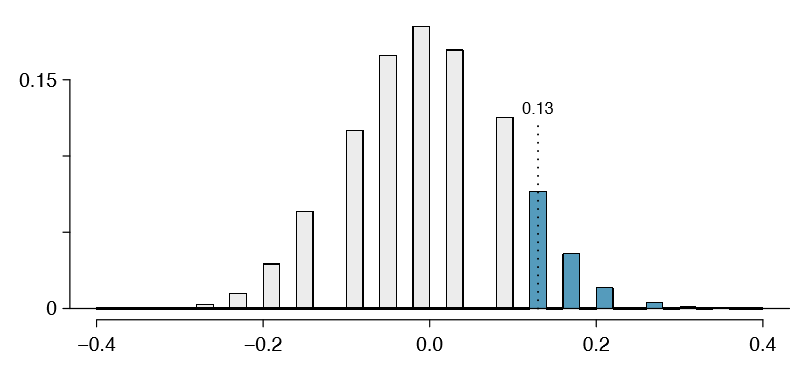
We build up an approximation to the null distribution by repeatedly creating tables like the one shown in Table 6.24 and computing the sample differences. The null distribution from 10,000 simulations is shown in Figure 6.25.
Example \(\PageIndex{4}\)
Compare Figures 6.23 and 6.25. How are they similar? How are they different?
Solution
The shapes are similar, but the simulated results show that the continuous approximation of the normal distribution is not very good. We might wonder, how close are the p-values?

Exercise \(\PageIndex{3}\)
The right tail area is about 0.13. (It is only a coincidence that we also have \(\hat {p}_t - \hat {p}_c = 0.13\).) The p-value is computed by doubling the right tail area: 0.26. How does this value compare with the large sample approximation for the p-value?
Solution
The approximation in this case is fairly poor (p-values: 0.174 vs. 0.26), though we come to the same conclusion. The data do not provide convincing evidence showing the blood thinner helps or hurts patients.
In general, small sample methods produce more accurate results since they rely on fewer assumptions. However, they often require some extra work or simulations. For this reason, many statisticians use small sample methods only when conditions for large sample methods are not satisfied.
Randomization for two-way tables and chi-square
Randomization methods may also be used for the contingency tables. In short, we create a randomized contingency table, then compute a chi-square test statistic \(X^2_{sim}\). We repeat this many times using a computer, and then we examine the distribution of these simulated test statistics. This randomization approach is valid for any sized sample, and it will be more accurate for cases where one or more expected bin counts do not meet the minimum threshold of 5. When the minimum threshold is met, the simulated null distribution will very closely resemble the chi-square distribution. As before, we use the upper tail of the null distribution to calculate the p-value.


