
6: Confidence Intervals and Sample Size
- Page ID
- 5323

The inferences that were discussed in chapters 5 and 6 were based on the assumption of an a priori hypothesis that the researcher had about a population. However, there are times when the researchers do not have a hypothesis. In such cases they would simply like a good estimate of the parameter.
By now you should realize that the statistic (which comes from the sample) will most likely not equal the parameter of the population, but it will be relatively close since it is part of the normally distributed collection of possible statistics. Consequently, the best that can be claimed is that the statistic is a point estimate of the parameter. Because half the statistics that could be selected are higher than the parameter and half are lower, and because the variation that can be expected for statistics is dependent, in part, upon sample size, then the knowledge of the statistic is insufficient for determining the degree to which it is a good estimate for the parameter. For this reason, estimates are provided with confidence intervals instead of point estimates.
You are probably most familiar with the concept of confidence intervals from polling results preceding elections. A reporter might say that 48% of the people in a survey plan to vote for candidate A, with a margin of error of plus or minus 3%. The interpretation is that between 45% and 51% of the population of voters will vote for candidate A. The size of the margin of error provides information about the potential gap between the point estimate (statistic) and the parameter. The interval gives the range of values that is most likely to contain the true parameter. For a confidence interval of (0.45,0.51) the possibility exists that the candidate could have a majority of the support. The margin of error, and consequently the interval, is dependent upon the degree of confidence that is desired, the sample size, and the standard error of the sampling distribution.
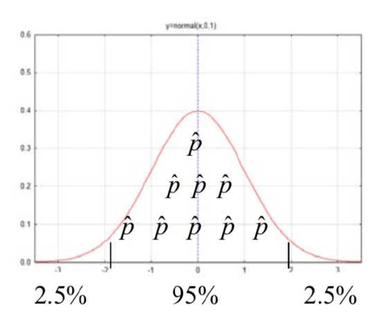
The logic behind the creation of confidence intervals can be demonstrated using the empirical rule, otherwise known as the 68-95-99.7 rule that you learned in Chapter 5. We know that of all the possible statistics that comprise a sampling distribution, 95% of them are within approximately 2 standard errors of the mean of the distribution. From this we can deduce that the mean of the distribution is within 2 standard errors of 95% of the possible statistics. By analogy, this is equivalent to saying that if you are less than two meters from the student who is seated next to you, then that student is less than two meters from you. Consequently, by taking the statistic and adding and subtracting two standard errors, an interval is created that should contain the parameter for 95% of the statistics we could get using a good random sampling process.
When using the empirical rule, the number 2, in the phrase “2 standard errors”, is called a critical value. However, a good confidence interval requires a critical value with more precision than is provided by the empirical rule. Furthermore, there may be a desire to have the degree of confidence be something besides 95%. Common alternatives include 90% and 99% confidence intervals. If the degree of confidence is 95%, then the critical values separate the middle 95% of the possible statistics from the rest of the distribution. If the degree of confidence is 99%, then the critical values separate the middle 99% of the possible statistics from the rest of the distribution. Whether the critical value is found in the standard normal distribution (a \(z\) value) or in the t distributions (a t value) is based on the whether the confidence interval is for a proportion or a mean.
The critical value and the standard error of the sampling distribution must be determined in order to calculate the margin of error.
The critical value is found by first determining the area in one tail. The area in the left tail (AL) is found by subtracting the degree of confidence from 1 and then dividing this by 2.
\[A_L = \dfrac{1 - \text{degree of confidence}}{2}.\]
For example, substituting into the formula for a 95% confidence interval produces
\[A_L = \dfrac{1 - 0.95}{2} = 0.025\]
The critical Z value for an area to the left of 0.025 is -1.96. Because of symmetry, the critical value of an area to the right of 0.025 is +1.96. This means that if we find the critical values corresponding to an area in the left tail of 0.025, that we will find the lines that separate the group of statistics with a 95% chance of being selected from the group that has a 5% chance of being selected.
An area in the left tail of 0.025, which is found in the body of the z distribution table, corresponds with a \(z^{\ast}\) value of -1.96. This is shown in the section of the Z table shown below.
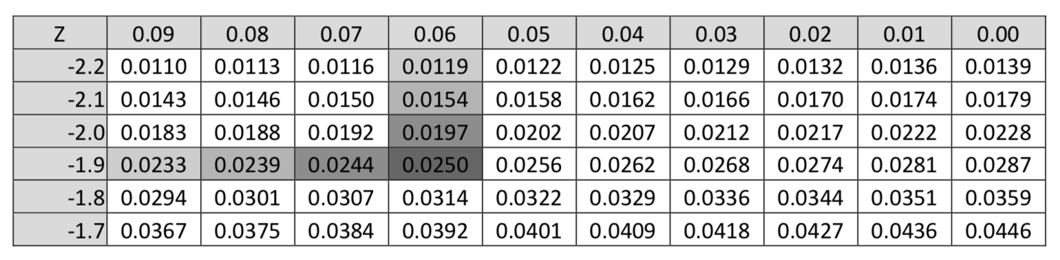
The critical \(z\) value of -1.96 is also called the 2.5th percentile. That means that 2.5% of all possible statistics are below that value.
Critical values can also be found using a TI 84 calculator. Use \(2^{\text{nd}}\) Distr, #3 invnorm (percentile, \(\mu\), \(\sigma\)). For example invnorm(0.025,0,1) gives -1.95996 which rounds to -1.96.
Confidence intervals for proportions always have a critical value found on the standard normal distribution. The \(z\) value that is found is given the notation \(z^{\ast}\). These critical values vary based on the degree of confidence. The other most common confidence intervals are 90% and 99%. Complete the following table below to find these commonly used critical values.
| Degree of Confidence | Area in Left Tail | \(z^{\ast}\) |
|---|---|---|
| 0.90 | ||
| 0.95 | 0.025 | 1.96 |
| 0.99 |
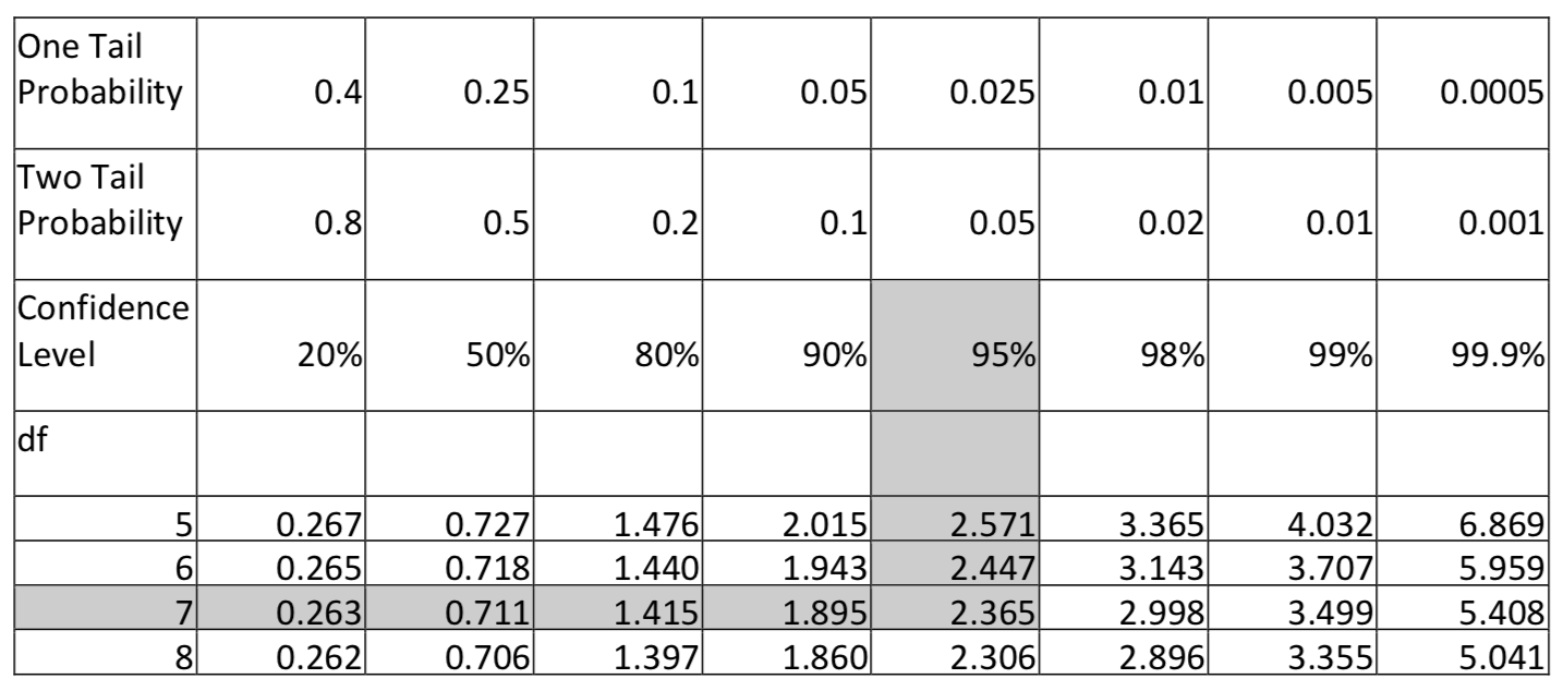
Confidence intervals for means require a critical value, \(t^{\ast}\), which is found on the t tables. These critical values are dependent upon both the degree of confidence and the sample size, or more precisely, the degrees of freedom. The top of the t-table provides a variety of confidence levels along with the area in one or both tails. The easiest approach to finding the critical \(t^{\ast}\) value is to find the column with the appropriate confidence level then find where that column intersects with the row containing the appropriate degrees of freedom. For example, the \(t^{\ast}\) value for a 95% confidence interval with 7 degrees of freedom is 2.365.
The second component of the margin of error, which is the standard error for the sampling distribution, assumes knowledge of the mean of the distribution (e.g. \(\mu_{\hat{p}} = p\) and \(\mu_{\bar{x}} = \mu\)). When testing hypotheses about the mean of the distribution, we assume these values because we assume the null hypothesis is true. However, when creating confidence intervals, we admit to not knowing these values and so consequently we cannot use the standard error. For example, the standard error for the \(\sigma_{\hat{p}} = \sqrt{\dfrac{p(1 - p)}{n}}\). Since we don’t know \(p\), we can’t use this formula. Likewise, the standard error for the distribution of sample means is \(\sigma_{\bar{x}} = \dfrac{\sigma}{\sqrt{n}}\). To find \(\sigma\) we need to know the population mean, \(\mu\), but once again we don’t know it, and we don’t even have a hypothesis about it, so consequently we can’t find \(\sigma\). The strategy in both these cases is to find an estimate of the standard error by using a statistic to estimate the missing parameter. Thus, \(\hat{p}\) is used to estimate \(p\) and \(s\) is used to estimate \(\sigma\). The estimated standard errors then become: \(s_{\hat{p}} = \sqrt{\dfrac{\hat{p}(1 - \hat{p})}{n}}\) and \(s_{\bar{x}} = \dfrac{s}{\sqrt{n}}\).
The groundwork has now been laid to develop the confidence interval formulas for the situations for which we tested hypotheses in the preceding chapter, namely \(p\), \(p_A - p_B\), \(\mu\), and \(\mu_A - \mu_B\). The table below summarizes these four parameters, their distributions and estimated standard errors.
| Parameter | Distribution | Estimated Standard Error |
|---|---|---|
| Proportion for one population, \(p\) | 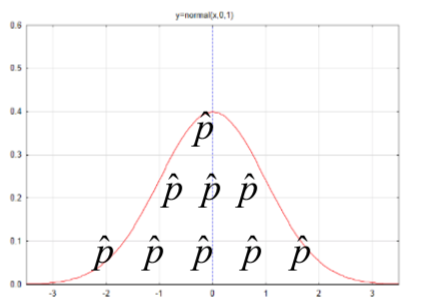 |
\(s_{\hat{p}} = \sqrt{\dfrac{\hat{p}(1 - \hat{p})}{n}}\) |
| Difference between proportions for two populations, \(p_A - p_B\) | 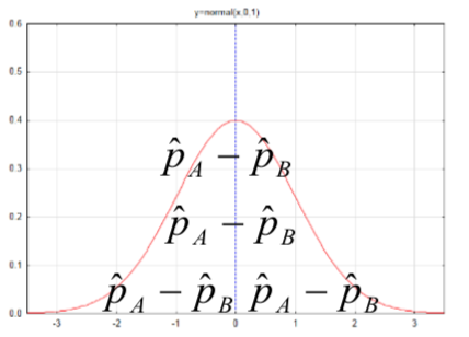 |
\(s_{\bar{p}_A - \bar{p}_B} = \sqrt{\dfrac{\hat{p}_A(1 - \hat{p}_A)}{n_A} + \dfrac{\hat{p}_B(1 - \hat{p}_B)}{n_B}}\) |
| Mean for one population or mean difference for dependent data, \(\mu\) | 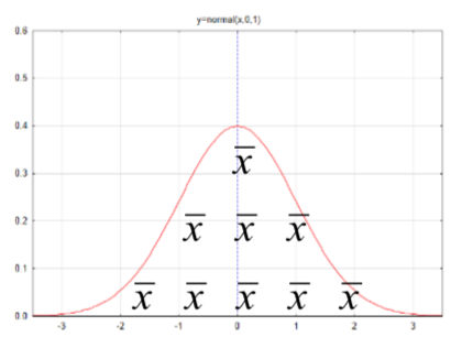 |
\(s_{\bar{x}} = \dfrac{s}{\sqrt{n}}\) |
| Difference between means of two independent populations, \(\mu_A - \mu_B\) | 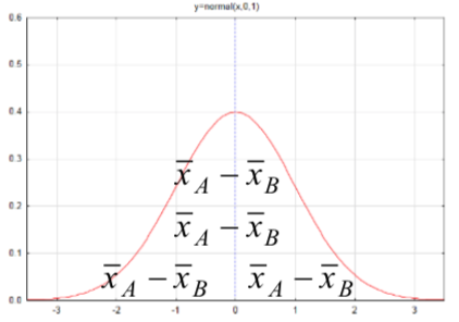 |
\(s_{\bar{x}_A - \bar{x}_B} = \sqrt{[\dfrac{(n_A - 1) s_{A}^{2} + (n_B - 1) s_{B}^{2}}{n_A + n_B - 2}][\dfrac{1}{n_A} + \dfrac{1}{n_B}]}\) |
The reasoning process for determining the formulas for the confidence intervals is the same in all cases.
- Determine the degree of confidence. The most common are 95%, 99% and 90%.
- Use the degree of confidence along with the appropriate table (z* or t*) to find the critical value.
- Multiply the critical value times the standard error to find the margin of error.
- The confidence interval is the statistic plus or minus the margin of error.
Notice that all the confidence intervals have the same format, even though some look more difficult than others.
statistic \(\pm\) margin of error
statistic \(\pm\) critical value \(\times\) estimated standard error
Confidence intervals about the proportion for one population:
\[\hat{p} \pm z^{\ast} \sqrt{\hat{p}(1 - \hat{p})}{n}\]
Confidence intervals for the difference in proportions between two populations:
\[(\hat{p}_A - \hat{p}_B \pm z^{\ast} \sqrt{\dfrac{\hat{p}_A\hat{q}_A}{n_A} + \dfrac{\hat{p}_B\hat{q}_B}{n_B}}\]
Remember that \(q = 1 – p\).
Confidence intervals for the mean for one population:
\[\bar{x} \pm t^{\ast} \dfrac{s}{\sqrt{n}}\]
Confidence interval for the difference between two independent mean:
\[(\bar{x}_A + \bar{x}_B \pm t^{\ast} (\sqrt{[\dfrac{(n_A - 1) s_{A}^{2} + (n_B - 1) s_{B}^{2}}{n_A + n_B - 2}][\dfrac{1}{n_A} + \dfrac{1}{n_B}]})\]
where \(t^{\ast}\) is the appropriate percentile from the t(\(n_A\) + \(n_B\) - 2) distribution.
The confidence interval formulas are organized below in the same way the hypothesis test formulas were organized in Chapter 6. You should see a similarity between corresponding formulas.
| Proportions (for categorical data) | Means (for quantitative data) | |
|---|---|---|
| 1 - sample |
\(\hat{p} \pm z^{\ast} \sqrt{\hat{p}(1 - \hat{p})}{n}\) Assumptions: \(np \ge 5\), \(n(1-p) \ge 5\) |
\(\bar{x} \pm t^{\ast} \dfrac{s}{\sqrt{n}}\) df = n - 1 Assumptions: If \(n < 30\), population is approximately normally distributed. |
| 2 - samples |
\((\hat{p}_A - \hat{p}_B \pm z^{\ast} \sqrt{\dfrac{\hat{p}_A\hat{q}_A}{n_A} + \dfrac{\hat{p}_B\hat{q}_B}{n_B}}\) Assumption: \(np \ge 5\), \(n(1-p) \ge 5\) for both population |
\((\bar{x}_A + \bar{x}_B \pm t^{\ast} (\sqrt{[\dfrac{(n_A - 1) s_{A}^{2} + (n_B - 1) s_{B}^{2}}{n_A + n_B - 2}][\dfrac{1}{n_A} + \dfrac{1}{n_B}]})\) df = \(n_A\) + \(n_B\) - 2 Assumptions: If \(n < 30\), population is approximately normally distributed. |
What does a confidence interval mean? For a 95% confidence interval, 95% of all possible statistics are within z* (or t*) standard errors of the mean of the distribution. Therefore, there is a 95% probability that the data that is randomly selected will produce one of those statistics and the confidence interval that is created will contain the parameter. Whether the interval ultimately does include the parameter or not is unknown. We only know that if the sampling processes was repeated a large number of times producing many confidence intervals, about 95% of them would contain the parameter.
Example 1
In an automaticity experiment community college students were given two opportunities to go to the computer lab to test their automaticity skills (math fact fluency). Students were randomly assigned to use one of two practice programs to determine if one program leads to greater improvement than the other. These programs will be called program A and program B.
a. What is the 95% confidence interval for the proportion of students who improve from their first attempt to their second attempt if 99 out of 113 students improved?
To help pick the correct confidence interval formula, notice this problem is about proportions and there is only one group of student.
The formula that meets these criteria is: \(\hat{p} \pm z^{\ast} \sqrt{\hat{p}(1 - \hat{p})}{n}\). Before substituting, it is necessary to calculate \(\hat{p}\). Since \(\hat{p} = \dfrac{x}{n} = \dfrac{99}{113} = 0.876\) (round to 3 decimal places), then the confidence interval formula becomes \(0.876 \pm 1.96 \sqrt{\dfrac{0.876(1 - 0.876}{113}}\). This simplifies to 0.876 \(\pm\) 0.061. The margin of error is 6.1%. The confidence interval is (0.815,0.937). The conclusion is that we are 95% confident that the true proportion of students who would improve from one test to the next is between 0.815 (81.5%) and 0.937 (93.7%).
To find this interval on the TI 84 calculator, select Stat, Tests, A 1-PropZInt.
b. What is the 90% confidence interval for the difference in the proportion of students who improved from their first attempt to their second attempt using Program A (37/45) and Program B (61/67)?
To help pick the correct confidence interval formula, notice this problem is about proportions and there are two different populations – one using Program A and the other using Program B.
The formula that meets these criteria is: \((\hat{p}_A - \hat{p}_B \pm z^{\ast} \sqrt{\dfrac{\hat{p}_A\hat{q}_A}{n_A} + \dfrac{\hat{p}_B\hat{q}_B}{n_B}}\). Since \(\hat{p}_A = \dfrac{x}{n} = \dfrac{37}{45} = 0.822\) and \(\hat{p}_B = \dfrac{x}{n} = \dfrac{61}{67} = 0.919\), then the confidence interval formula becomes
\(0.822 - 0.910) \pm 1.645 \sqrt{\dfrac{0.822(1 - 0.822)}{45} + \dfrac{0.910(1 - 0.910)}{67}}\)
After simplification the confidence interval can be written as a statistic ± margin of error: -0.088 \(\pm\) 0.110. The margin of error is 11.0%. The confidence interval is (-0.198,0.022). The conclusion is that we are 90% confident that the true difference in proportions between those using Program A and those using Program B is between -0.198 and 0.022. Notice that 0 falls within that range, which indicates there is potentially no difference between these two proportions.
To find this interval on the TI 84 calculator, select Stat, Tests, B 2-PropZInt.
c. What is the 99% confidence interval for the average improvement from Introductory Algebra students using program B (mean = 5.0, SD = 3.18, n = 19).
To help pick the correct confidence interval formula, notice this problem is about means and there is only one population (Introductory Algebra students using program B).
The formula that meets these criteria is: \(\bar{x} \pm t^{\ast} \dfrac{s}{\sqrt{n}}\). There are 18 degrees of freedom (df = n-1) so the \(t^{\ast}\) value is 2.878. After substituting for all the variables the formula becomes \(5.0 \pm 2.878 \dfrac{3.18}{\sqrt{19}}\). This simplifies to 5.0 \(\pm\) 2.1. The confidence interval is (2.9, 7.1).
To find this interval on the TI 84 calculator, select Stat, Tests, #8 Tinterval.
d. What is the 95% confidence for the difference in improvement between introductory algebra and intermediate algebra students using program A. The statistics for introductory algebra are mean = 2.4, SD = 3.53, n = 16. The statistics for intermediate algebra are mean = 4, SD = 4.89, n = 21.
To help pick the correct confidence interval formula, notice this problem is about means but there are two populations (introductory algebra students and intermediate algebra students). The formula that meets these criteria is:
\((\bar{x}_A + \bar{x}_B \pm t^{\ast} (\sqrt{[\dfrac{(n_A - 1) s_{A}^{2} + (n_B - 1) s_{B}^{2}}{n_A + n_B - 2}][\dfrac{1}{n_A} + \dfrac{1}{n_B}]})\)
There are 35 degrees of freedom (\(n_A\) + \(n_B\) - 2). Unfortunately, this value does not exist on the \(t\) table in Chapter 6, so it will be necessary to estimate it. One approach is to use the critical value for 30 degrees of freedom (2.042) which is larger than the critical value for 40 degrees of freedom (2.021) as this will ensure that the confidence interval is at least as large as necessary. After substituting for all the variables, the formula becomes \((2.4 - 4) \pm 2.042 (4.359 \sqrt{\dfrac{1}{16} + \dfrac{1}{21}})\) and with simplification -1.6 \(\pm\) 2.95. The interval is (-4.55,1.35). Because the critical \(t^{\ast}\) value is slightly larger than it should be, the interval is slightly wider than it would be calculated using the functions on a TI 84 calculator (-4.537,1.3368).
The second approach is to find this interval on the TI 84 calculator. Select Stat, Tests, #0 2-SampTInt.
Sample Size Estimation
The margin of error portion of a confidence interval formula can also be used to estimate the sample size that needed. Let E represent the desired margin of error. If sampling of categorical data for one population is done, then \(E = z^{\ast} \sqrt{\dfrac{\hat{p}(1 - \hat{p})}{n}}\). Solve this for n using algebra. Since the goal is to make sure the sample size is large enough, and since \(\hat{p}\) is not known in advance, then it is necessary to make sure that \(\hat{p}(1 - \hat{p})\) is the largest possible value. That will happen when \(\hat{p} = 0.5\).
\(E = z^{\ast} \sqrt{\dfrac{\hat{p}(1 - \hat{p})}{n}}\)
\(\dfrac{E}{z^{\ast}} = \sqrt{\dfrac{\hat{p}(1 - \hat{p})}{n}}\)
\(\dfrac{E^2}{z^{\ast^{2}}} = \dfrac{\hat{p}(1 - \hat{p})}{n}\)
\(n = \dfrac{z^{\ast^{2}} \hat{p}(1 - \hat{p})}{E^2}\)
\(n = \dfrac{z^{\ast^{2}} 0.5(0.5)}{E^2}\)
\(n = \dfrac{0.25 z^{\ast^{2}}}{E^2}\) or \(n = \dfrac{z^{\ast^{2}}}{4E^2}\)
Example 2
Estimate the sample size needed for a national presidential poll if the desired margin of error is 3%. Assume 95% degree of confidence.
\(n = \dfrac{1.96^2}{4(0.03)^2} = 1067.1\) or 1068 (round up to get enough in the ample).