3.7: Changing data- basics of transformations

In complicated studies involving many data types: measurements and ranks, percentages and counts, parametric, nonparametric and nominal, it is useful to unify them. Sometimes such transformations are easy. Even nominal data may be understood as continuous, given enough information. For example, sex may be recorded as continuous variable of blood testosterone level, possibly with additional measurements. Another, more common way, is to treat discrete data as continuous—it is usually safe, but sometimes may lead to unpleasant surprises.

Another possibility is to transform measurement data into ranked. R function cut() allows to perform this operation and create ordered factors.

What is completely unacceptable is transforming common nominal data into ranks. If values are not, by their nature, ordered, imposing an artificial order can make the results meaningless.

Data are often transformed to make them closer to parametric and to homogenize standard deviations. Distributions with long tails, or only somewhat bell-shaped (as in Figure 4.2.5), might be log-transformed. It is perhaps the most common transformation.

There is even a special argument plot(..., log="axis"), where "axis" should be substituted with x or y, presenting it in (natural) logarithmic scale. Another variant is to simply calculate logarithm on the fly like plot(log(...).

Consider some widely used transformations and their implications in R(we assume that your measurements are recorded in the vector data):

• Logarithmic: log(data + 1). It may normalize distributions with positive skew (right-tailed), bring relationships between variables closer to linear and equalize variances. It cannot handle zeros, this is why we added a single digit.
• Square root: sqrt(data). It is similar to logarithmic in its effects, but cannot handle negatives.
• Inverse: 1/(data + 1). This one stabilizes variances, cannot handle zeros.
• Square: data^2. Together with square root, belongs to family of power transformations. It may normalize data with negative skew (left-tailed) data, bring relationships between variables closer to linear and equalize variances.
• Logit: log(p/(1-p)). It is mostly used on proportions to linearize S-shaped, or sigmoid, curves. Along with logit, these types of data are sometimes treated with arcsine transformation which is asin(sqrt(p)). In both cases, p must be between 0 and 1.

While working with multiple variables, keep track of their dimensions. Try not to mix them up, recording one variable in millimeters, and another in centimeters. Nevertheless, in multivariate statistics even data measured in common units might have different nature. In this case, variables are often standardized, e.g. brought to the same mean and/or the same variance with scale() function. Embedded trees data is a good example:

Code \(\PageIndex{1}\) (R):

scale(trees)

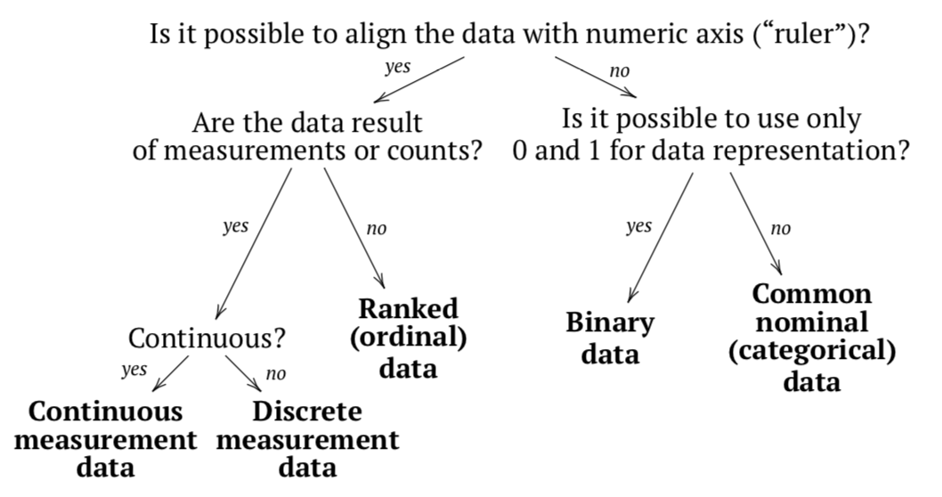
At the end of data types explanation, we recommend to review a small chart which could be helpful for the determination of data type (Figure \(\PageIndex{1}\)).

Figure \(\PageIndex{1}\) How to tell the kind of data.