7.7: Answers to exercises

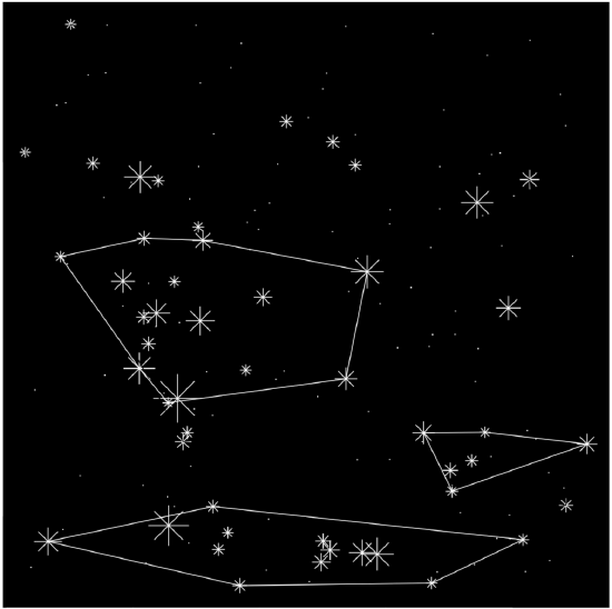
Answer to the stars question.

First, load the data and as suggested above, convert coordinates into decimals:

Code \(\PageIndex{1}\) (R):

s50 <- read.table("data/stars.txt", h=T, sep="	", as.is=T, quote="")
str(s50)
RA10 <- as.numeric(substr(s50$RA, 1, 2)) + as.numeric(substr(s50$RA, 4, 5))/60 +  as.numeric(substr(s50$RA, 7, 10))/3600
DEC10 <- sign(as.numeric(substr(s50$DEC, 1, 3))) *  (as.numeric(substr(s50$DEC, 2, 3)) +  as.numeric(substr(s50$DEC, 5, 6))/60 +  as.numeric(substr(s50$DEC, 8, 9))/3600)
coo <- cbind(RA10, DEC10)

Next, some preliminary plots (please make them yourself):

Code \(\PageIndex{2}\) (R):

s50 <- read.table("data/stars.txt", h=T, sep="	", as.is=T, quote="")
RA10 <- as.numeric(substr(s50$RA, 1, 2)) + as.numeric(substr(s50$RA, 4, 5))/60 + as.numeric(substr(s50$RA, 7, 10))/3600
DEC10 <- sign(as.numeric(substr(s50$DEC, 1, 3)))*(as.numeric(substr(s50$DEC, 2, 3))+as.numeric(substr(s50$DEC, 5, 6))/60+as.numeric(substr(s50$DEC, 8, 9))/3600
coo <- cbind(RA10, DEC10)
oldpar <- par(bg="black", fg="white", mar=rep(0, 4))
plot(coo, pch="*", cex=(3 - s50$VMAG))
Hulls(coo, as.numeric(factor(s50$CONSTEL)), # asmisc.r usecolors=rep("white", nlevels(factor(s50$CONSTEL))))
points(runif(100, min(RA10), max(RA10)), runif(100, min(DEC10), max(DEC10)), pch=".")
par(oldpar)
plot(coo, type="n")
text(coo, s50$CONSTEL.A)
plot(coo, type="n")
text(coo, s50$NAME)

Now, load dbscan package and try to find where number of “constellations” is maximal:

Code \(\PageIndex{3}\) (R):

library(dbscan)
s50 <- read.table("data/stars.txt", h=T, sep="	", as.is=T, quote="")
RA10 <- as.numeric(substr(s50$RA, 1, 2)) + as.numeric(substr(s50$RA, 4, 5))/60 +  as.numeric(substr(s50$RA, 7, 10))/3600
DEC10 <- sign(as.numeric(substr(s50$DEC, 1, 3)))*(as.numeric(substr(s50$DEC, 2, 3))+as.numeric(substr(s50$DEC, 5, 6))/60+as.numeric(substr(s50$DEC, 8, 9))/3600
coo <- cbind(RA10, DEC10)
for (eps in 1:20) cat(c(eps, ":", names(table(dbscan(coo, eps=eps)$cluster))), "
")

Plot the prettified “night sky” (Figure \(\PageIndex{1}\)) with found constellations:

Code \(\PageIndex{4}\) (R):

library(dbscan)
s50 <- read.table("data/stars.txt", h=T, sep="	", as.is=T, quote="")
RA10 <- as.numeric(substr(s50$RA, 1, 2)) + as.numeric(substr(s50$RA, 4, 5))/60 +  as.numeric(substr(s50$RA, 7, 10))/3600
DEC10 <- sign(as.numeric(substr(s50$DEC, 1, 3)))*(as.numeric(substr(s50$DEC, 2, 3))+as.numeric(substr(s50$DEC, 5, 6))/60+as.numeric(substr(s50$DEC, 8, 9))/3600
coo <- cbind(RA10, DEC10)
s50.db <- dbscan(coo, eps=9)
oldpar <- par(bg="black", fg="white", mar=rep(0, 4))
plot(coo, pch=8, cex=(3 - s50$VMAG))
Hulls(coo, s50.db$cluster, # asmisc.r usecolors=c("black", "white", "white", "white"))
points(runif(100, min(RA10), max(RA10)),  runif(100, min(DEC10), max(DEC10)), pch=".")
par(oldpar)

dev.off()

To access agreement between two classifications (two systems of constellations) we might use adjusted Rand index which counts correspondences:

Figure \(\PageIndex{1}\) Fifty brightest stars with “constellations” found with DBSCAN.

Code \(\PageIndex{5}\) (R):

s50 <- read.table("data/stars.txt", h=T, sep="	", as.is=T, quote="")
library(dbscan)
RA10 <- as.numeric(substr(s50$RA, 1, 2)) + as.numeric(substr(s50$RA, 4, 5))/60 +  as.numeric(substr(s50$RA, 7, 10))/3600
DEC10 <- sign(as.numeric(substr(s50$DEC, 1, 3)))*(as.numeric(substr(s50$DEC, 2, 3))+as.numeric(substr(s50$DEC, 5, 6))/60+as.numeric(substr(s50$DEC, 8, 9))/3600
coo <- cbind(RA10, DEC10)
s50.db <- dbscan(coo, eps=9)
Adj.Rand(as.numeric(factor(s50$CONSTEL)), s50.db$cluster) # asmisc.r

(It is of course, low.)

Answer to the beer classification exercise. To make hierarchical classification, we need first to make the distance matrix. Let us look on the data:

Code \(\PageIndex{6}\) (R):

beer <- read.table("data/beer.txt", sep="	", h=TRUE)
head(beer)

Data is binary and therefore we need the specific method of distance calculation. We will use here Jaccard distance implemented in vegdist() function from the vegan package. It is also possible to use here other methods like “binary” from the core dist() function. Next step would be the construction of dendrogram (Figure \(\PageIndex{2}\)):

Code \(\PageIndex{7}\) (R):

beer <- read.table("data/beer.txt", sep="	", h=TRUE)
library(vegan)
beer.d <- vegdist(beer, "jaccard")
plot(hclust(beer.d, method="ward.D"), main="", xlab="", sub="")

Figure \(\PageIndex{2}\) Hierarchical classification of Russian beer types.

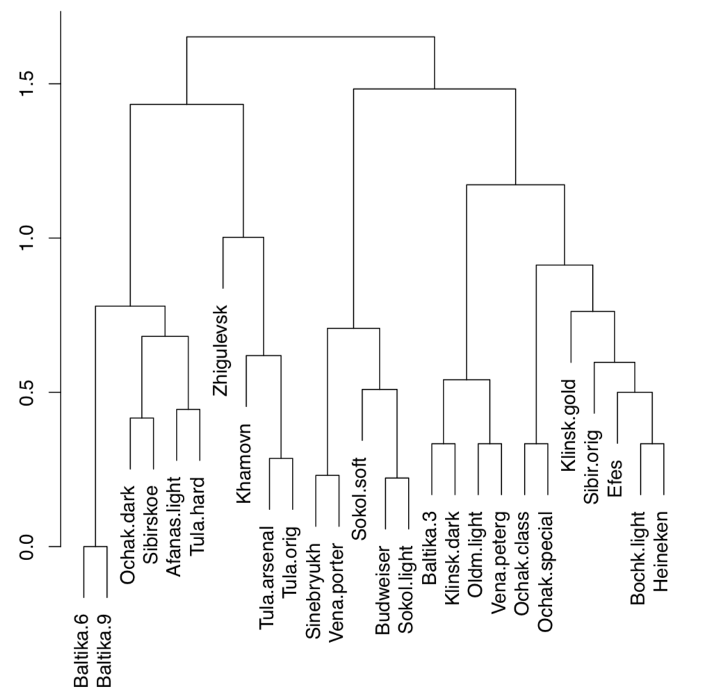
There are two big groups (on about 1.7 dissimilarity level), we can call them “Baltika” and “Budweiser”. On the next split (approximately on 1.4 dissimilarity), there are two subgroups in each group. All other splits are significantly deeper. Therefore, it is possible to make the following hierarchical classification:

• Baltika group
  • Baltika subgroup: Baltika.6, Baltika.9, Ochak.dark, Afanas.light, Sibirskoe, Tula.hard
  • Tula subgroup: Zhigulevsk, Khamovn, Tula.arsenal, Tula.orig
• Budweiser group
  • Budweiser subgroup: Sinebryukh, Vena.porter, Sokol.soft, Budweiser, Sokol.light
  • Ochak subgroup: Baltika.3, Klinsk.dark, Oldm.light, Vena.peterg, Ochak.class, Ochak.special, Klinsk.gold, Sibir.orig, Efes, Bochk.light, Heineken

It is also a good idea to check the resulted classification with any other classification method, like non-hierarchical clustering, multidimensional scaling or even PCA. The more consistent is the above classification with this second approach, the better.

Answer to the plant species classification tree exercise. The tree is self-explanatory but we need to build it first (Figure \(\PageIndex{3}\)):

Code \(\PageIndex{8}\) (R):

eq <- read.table("data/eq.txt", h=TRUE)
eq.tree <- tree(eq[, 1] ~ ., eq[,-1])
plot(eq.tree); text(eq.tree)

Answer to the kubricks (Figure \(\PageIndex{3}\)) question. This is just a plan as you will still need to perform these steps individually:

1. Open R, open Excel or any spreadsheet software and create the data file. This data file should be the table where kubrick species are rows and characters are columns (variables). Every row should start with a name of kubrick (i.e., letter), and every column should have a header (name of character). For characters, short uppercased names with no spaces are preferable.

Figure \(\PageIndex{3}\) Classification tree shows that two horsetail species differ by N.REB character (number of stem ridges)

Topleft cell might stay empty. In every other cell, there should be either 1 (character present) or 0 (character absent). For the character, you might use “presence of stalk” or “presence of three mouths”, or “ability to make photosynthesis”, or something alike. Since there are 8 kubricks, it is recommended to invent \(N+1\) (in this case, 9) characters.

2. Save your table as a text file, preferably tab-separated (use approaches described in the second chapter), then load it into R with read.table(.., h=TRUE, row.names=1).

3. Apply hierarchical clustering with the distance method applicable for binary (0/1) data, for example binary from dist() or another method (like Jaccard) from the vegan::vegdist().

4. Make the dendrogram with hclust() using the appropriate clustering algorithm.

In the data directory, there is a data file, kubricks.txt. It is just an example so it is not necessarily correct and does not contain descriptions of characters. Since it is pretty obvious how to perform hierarchical clustering (see the “beer” example above), we present below two other possibilities.

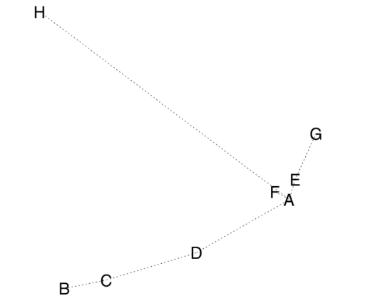
First, we use MDS plus the MST, minimum spanning tree, the set of lines which show the shortest path connecting all objects on the ordination plot (Figure \(\PageIndex{4}\)):

Code \(\PageIndex{9}\) (R):

kubricks <- read.table("data/kubricks.txt", h=TRUE, row.names=1)
kubricks.d <- dist(kubricks, method="binary")
kubricks.c <- cmdscale(kubricks.d)
plot(kubricks.c, type="n", axes=FALSE)
text(kubricks.c, labels=row.names(kubricks), cex=2)
library(vegan)
lines(spantree(kubricks.d), kubricks.c[, 1:2], lty=2)

Figure \(\PageIndex{4}\) Minimum spanning tree of kubricks.

Second, we can take into account that kubricks are biological objects. Therefore, with the help of packages ape and phangorn we can try to construct the most parsimonious (i.e., shortest) phylogeny tree for kubricks. Let us accept that kubrick H is the outgroup, the most primitive one:

Code \(\PageIndex{10}\) (R):

kubricks <- read.table("data/kubricks.txt", h=TRUE, row.names=1)
library(phangorn)
k <- as.phyDat(data.frame(t(kubricks)), type="USER", levels = c(0, 1))
kd <- dist.hamming(k) # Hamming distance for morphological data
kdnj <- NJ(kd) # neighbor-joining tree
kp <- optim.parsimony(kdnj, k)
ktree <- root(kp, outgroup="H", resolve.root=TRUE) # re-root
plot(ktree, cex=2)

(Make and review this plot yourself.)