5.3: If there are More than Two Samples - ANOVA

One way

What if we need to know if there are differences between three samples? The first idea might be to make the series of statistical tests between each pair of the sample. In case of three samples, we will need three t-tests or Wilcoxon tests. What is unfortunate is that number of required tests will grow dramatically with the number of samples. For example, to compare six samples we will need to perform 15 tests!

Even more serious problem is that all tests are based on the idea of probability. Consequently, the chance to make of the Type I error (false alarm) will grow every time we perform more simultaneous tests on the same sample.

For example, in one test, if null hypothesis is true, there is usually only a 5% chance to reject it by mistake. However, with 20 tests (Figure E.2), if all corresponding null hypotheses are true, the expected number of incorrect rejections is 1! This is called the problem of multiple comparisons.

One of most striking examples of multiple comparisons is a “dead salmon case”. In 2009, group of researches published results of MRI testing which detected the brain activity in a dead fish! But that was simply because they purposely did not account for multiple comparisons\(^{[1]}\).

The special technique, ANalysis Of VAriance (ANOVA) was invented to avoid multiple comparisons in case of more than two samples.

In R formula language, ANOVA might be described as

response ~ factor

where response is the measurement variable. Note that the only difference from two-sample case above is that factor in ANOVA has more then two levels.

The null hypothesis here is that all samples belong to the same population (“are not different”), and the alternative hypothesis is that at least one sample is divergent, does not belong to the same population (“samples are different”).

In terms of p-values:

Figure \(\PageIndex{1}\) explains it on example of multiple apple samples mixed with divergent tomato sample.

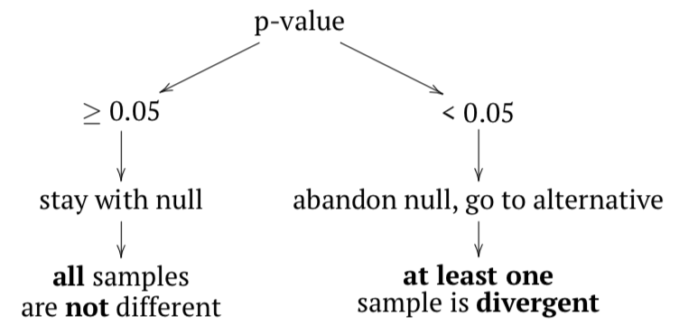
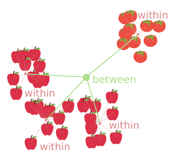
If any sample came from different population, then variance between samples should be at least comparable with (or larger then) variation within samples; in other words, F-value (or F-ratio) should be \(\geq 1\). To check that inferentially, F-test is applied. If p-value is small enough, then at least one sample (subset, column) is divergent.

ANOVA does not reveal which sample is different. This is because variances in ANOVA are pooled. But what if we still need to know that? Then we should apply post hoc tests. In is not required to run them after ANOVA; what is required is to perform them carefully and always apply p-value adjustment for multiple comparisons. This adjustment typically increases p-value to avoid accumulation from multiple tests. ANOVA and post hoc tests answer different research questions, therefore this is up to the researcher to decide which and when to perform.

ANOVA is a parametric method, and this typically goes well with its first assumption, normal distribution of residuals (deviations between observed and expected values). Typically, we check normality of the whole dataset because ANOVA uses pooled data anyway. It is also possible to check normality of residuals directly (see below). Please note that ANOVA tolerates mild deviations from normality, both in data and in residuals. But if the data is clearly nonparametric, it is recommended to use other methods (see below).

Figure \(\PageIndex{1}\) Core idea of ANOVA: compare within and between variances.

Second assumption is homogeinety of variance (homoscedasticity), or, simpler, similarity of variances. This is more important and means that sub-samples were collected with similar methods.

Third assumption is more general. It was already described in the first chapter: independence of samples. “Repeated measurements ANOVA” is however possible, but requires more specific approach.

All assumptions must be checked before analysis.

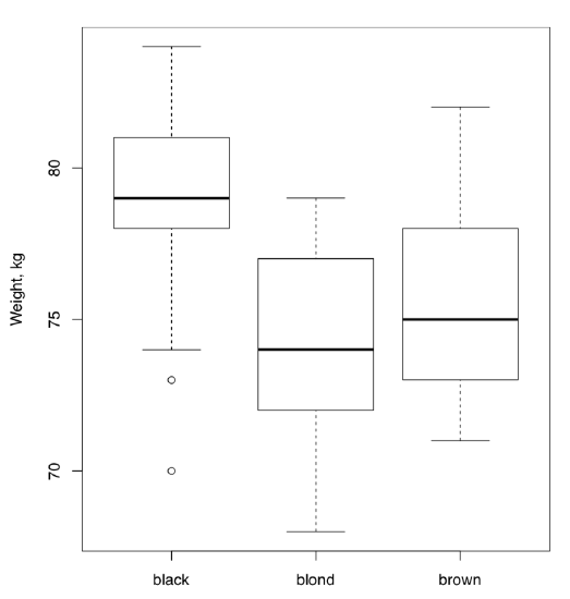
The best way of data organization for the ANOVA is the long form explained above: two variables, one of them contains numerical data, whereas the other describes grouping (in R terminology, it is a factor). Below, we create the artificial data which describes three types of hair color, height (in cm) and weight (in kg) of 90 persons:

Code \(\PageIndex{1}\) (R):

hwc <- read.table("data/hwc.txt", h=TRUE)
str(hwc)
boxplot(WEIGHT ~ COLOR, data=hwc, ylab="Weight, kg")

​​​(Note that notches and other “bells and whistles” do not help here because we want to estimate joint differences; raw boxplot is probably the best choice.)

Code \(\PageIndex{2}\) (R):

hwc <- read.table("data/hwc.txt", h=TRUE)
Normality <- function(a) {ifelse(shapiro.test(a)$p.value < 0.05, "NOT NORMAL", "NORMAL")}
sapply(hwc[sapply(hwc, is.numeric)], Normality) # asmisc.r
tapply(hwc$WEIGHT, hwc$COLOR, var)

(Note the use of double sapply() to check normality only for measurement columns.)

It looks like both assumptions are met: variance is at least similar, and variables are normal. Now we run the core ANOVA:

Code \(\PageIndex{3}\) (R):

hwc <- read.table("data/hwc.txt", h=TRUE)
wc.aov <- aov(WEIGHT ~ COLOR, data=hwc)
summary(wc.aov)

This output is slightly more complicated then output from two-sample tests, but contains similar elements (from most to least important):

1. p-value (expressed as Pr(>F)) and its significance;

2. statistic (F value);

3. degrees of freedom (Df)

All above numbers should go to the report. In addition, there are also:

1. variance within columns (Sum Sq for Residuals);

2. variance between columns (Sum Sq for COLOR);

3. mean variances (Sum Sq divided by Df)

(Grand variance is just a sum of variances between and within columns.)

If degrees of freedom are already known, it is easy enough to calculate F value and p-value manually, step by step:

Code \(\PageIndex{4}\) (R):

hwc <- read.table("data/hwc.txt", h=TRUE)
df1 <- 2
df2 <- 87
group.size <- 30
(sq.between <- sum(tapply(hwc$WEIGHT, hwc$COLOR, function(.x) (mean(.x) - mean(hwc$WEIGHT))^2))*group.size)
(mean.sq.between <- sq.between/df1)
(sq.within <- sum(tapply(hwc$WEIGHT, hwc$COLOR, function(.x) sum((.x - mean(.x))^2))))
(mean.sq.within <- sq.within/df2)
(f.value <- mean.sq.between/mean.sq.within)
(p.value <- (1 - pf(f.value, df1, df2)))

Of course, R calculates all of that automatically, plus also takes into account all possible variants of calculations, required for data with another structure. Related to the above example is also that to report ANOVA, most researches list three things: two values for degrees of freedom, F value and, of course, p-value.

All in all, this ANOVA p-value is so small that H\(_0\) should be rejected in favor of the hypothesis that at least one sample is different. Remember, ANOVA does not tell which sample is it, but boxplots (Figure \(\PageIndex{2}\)) suggest that this might be people with black hairs.

To check the second assumption of ANOVA, that variances should be at least similar, homogeneous, it is sometimes enough to look on the variance of each group with tapply() as above or with aggregate():

Code \(\PageIndex{5}\) (R):

hwc <- read.table("data/hwc.txt", h=TRUE)
aggregate(hwc[,-1], by=list(COLOR=hwc[, 1]), var)

Figure \(\PageIndex{2}\) Is there a weight difference between people with different hair color? (Artificial data.)

But better is to test if variances are equal with, for example, bartlett.test() which has the same formula interface:

Code \(\PageIndex{6}\) (R):

hwc <- read.table("data/hwc.txt", h=TRUE)
bartlett.test(WEIGHT ~ COLOR, data=hwc)

(The null hypothesis of the Bartlett test is the equality of variances.)

Alternative is nonparametric Fligner-Killeen test:

Code \(\PageIndex{7}\) (R):

hwc <- read.table("data/hwc.txt", h=TRUE)
fligner.test(WEIGHT ~ COLOR, data=hwc)

(Null is the same as in Bartlett test.)

The first assumption of ANOVA could also be checked here directly:

Code \(\PageIndex{8}\) (R):

hwc <- read.table("data/hwc.txt", h=TRUE)
wc.aov <- aov(WEIGHT ~ COLOR, data=hwc)
Normality <- function(a) {ifelse(shapiro.test(a)$p.value < 0.05, "NOT NORMAL", "NORMAL")}
Normality(wc.aov$residuals)

Effect size of ANOVA is called \(\eta^2\) (eta squared). There are many ways to calculate eta squared but simplest is derived from the linear model (see in next sections). It is handy to define \(\eta^2\) as a function:

Code \(\PageIndex{9}\) (R):

Eta2 <- function(aov){summary.lm(aov)$r.squared}

and then use it for results of both classic ANOVA and one-way test (see below):

Code \(\PageIndex{10}\) (R):

Eta2 <- function(aov){summary.lm(aov)$r.squared}
hwc <- read.table("data/hwc.txt", h=TRUE)
wc.aov <- aov(WEIGHT ~ COLOR, data=hwc)
(ewc <- Eta2(wc.aov))
Mag(ewc) # asmisc.r

The second function is an interpreter for \(\eta^2\) and similar effect size measures (like \(r\) correlation coefficient or R\(^2\) from linear model).

If there is a need to calculate effect sizes for each pair of groups, two-sample effect size measurements like coefficient of divergence (Lyubishchev’s K) are applicable.

One more example of classic one-way ANOVA comes from the data embedded in R(make boxplot yourself):

Code \(\PageIndex{11}\) (R):

Normality <- function(a) {ifelse(shapiro.test(a)$p.value < 0.05, "NOT NORMAL", "NORMAL")}
Normality(chickwts$weight)
bartlett.test(weight ~ feed, data=chickwts)
boxplot(weight ~ feed, data=chickwts)
chicks.aov <- aov(weight ~ feed, data=chickwts)
summary(chicks.aov)
Eta2(chicks.aov)
Eta2 <- function(aov){summary.lm(aov)$r.squared}
Mag(Eta2(chicks.aov)) # asmisc.r

Consequently, there is a very high difference between weights of chickens on different diets.

If there is a goal to find the divergent sample(s) statistically, one can use post hoc pairwise t-test which takes into account the problem of multiple comparisons described above; this is just a compact way to run many t-tests and adjust resulted p-values:

Code \(\PageIndex{12}\) (R):

hwc <- read.table("data/hwc.txt", h=TRUE)
pairwise.t.test(hwc$WEIGHT, hwc$COLOR)

(This test uses by default the Holm method of p-value correction. Another way is Bonferroni correction explained below. All available ways of correction are accessible trough the p.adjust() function.)

Similar to the result of pairwise t-test (but more detailed) is the result of Tukey Honest Significant Differences test (Tukey HSD):

Code \(\PageIndex{13}\) (R):

hwc <- read.table("data/hwc.txt", h=TRUE)
wc.aov <- aov(WEIGHT ~ COLOR, data=hwc)
TukeyHSD(wc.aov)

Are our groups different also by heights? If yes, are black-haired still different?

Post hoc tests output p-values so they do not measure anything. If there is a need to calculate group-to-group effect sizes, two samples effect measures (like Lyubishchev’s K) are generally applicable. To understand pairwise effects, you might want to use the custom function pairwise.Eff() which is based on double sapply():

Code \(\PageIndex{14}\) (R):

hwc <- read.table("data/hwc.txt", h=TRUE)
pairwise.Eff(hwc$WEIGHT, hwc$COLOR, eff="cohen.d") # asmisc.r

Next example is again from the embedded data (make boxplot yourself):

Code \(\PageIndex{15}\) (R):

Normality <- function(a) {ifelse(shapiro.test(a)$p.value < 0.05, "NOT NORMAL", "NORMAL")}
Normality(PlantGrowth$weight)
bartlett.test(weight ~ group, data=PlantGrowth)
plants.aov <- aov(weight ~ group, data=PlantGrowth)
summary(plants.aov)
Eta2 <- function(aov){summary.lm(aov)$r.squared}
Eta2(plants.aov)
Mag(Eta2(plants.aov)) # asmisc.r
boxplot(weight ~ group, data=PlantGrowth)
with(PlantGrowth, pairwise.t.test(weight, group))

As a result, yields of plants from two treatment condition are different, but there is no difference between each of them and the control. However, the overall effect size if this experiment is high.

If variances are not similar, then oneway.test() will replace the simple (one-way) ANOVA:

Code \(\PageIndex{16}\) (R):

hwc2 <- read.table("data/hwc2.txt", h=TRUE)
boxplot(WEIGHT ~ COLOR, data=hwc2)
Normality <- function(a) {ifelse(shapiro.test(a)$p.value < 0.05, "NOT NORMAL", "NORMAL")}
sapply(hwc2[, 2:3], Normality) # asmisc.r
tapply(hwc2$WEIGHT, hwc2$COLOR, var)
bartlett.test(WEIGHT ~ COLOR, data=hwc2)
oneway.test(WEIGHT ~ COLOR, data=hwc2)
Eta2 <- function(aov){summary.lm(aov)$r.squared}
(e2 <- Eta2(aov(WEIGHT ~ COLOR, data=hwc2)))
Mag(e2)
pairwise.t.test(hwc2$WEIGHT, hwc2$COLOR) # most applicable post hoc

(Here we used another data file where variables are normal but group variances are not homogeneous. Please make boxplot and check results of post hoc test yourself.)

What if the data is not normal?

The first workaround is to apply some transformation which might convert data into normal:

Code \(\PageIndex{17}\) (R):

Normality <- function(a) {ifelse(shapiro.test(a)$p.value < 0.05, "NOT NORMAL", "NORMAL")}
Normality(InsectSprays$count) # asmisc.r
Normality(sqrt(InsectSprays$count))

However, the same transformation could influence variance:

Code \(\PageIndex{18}\) (R):

bartlett.test(sqrt(count) ~ spray, data=InsectSprays)$p.value

Frequently, it is better to use the nonparametric ANOVA replacement, Kruskall-Wallis test:

Code \(\PageIndex{19}\) (R):

hwc3 <- read.table("data/hwc3.txt", h=TRUE)
boxplot(WEIGHT ~ COLOR, data=hwc3)
sapply(hwc3[, 2:3], Normality) # asmisc.r
kruskal.test(WEIGHT ~ COLOR, data=hwc3)

(Again, another variant of the data file was used, here variables are not even normal. Please make boxplot yourself.)

Effect size of Kruskall-Wallis test could be calculated with \(\epsilon^2\):

Code \(\PageIndex{20}\) (R):

hwc3 <- read.table("data/hwc3.txt", h=TRUE)
Epsilon2 <- function(kw, n) # n is the number of cases{unname(kw$statistic/((n^2 - 1)/(n+1)))}
kw <- kruskal.test(WEIGHT ~ COLOR, data=hwc3)
Epsilon2(kw, nrow(hwc3))
Mag(Epsilon2(kw, nrow(hwc3))) # asmisc.r

The overall efefct size is high, it also visible well on the boxplot (make it yourself):

Code \(\PageIndex{21}\) (R):

hwc3 <- read.table("data/hwc3.txt", h=TRUE)
boxplot(WEIGHT ~ COLOR, data=hwc3)

To find out which sample is deviated, use nonparametric post hoc test:

Code \(\PageIndex{22}\) (R):

hwc3 <- read.table("data/hwc3.txt", h=TRUE)
pairwise.wilcox.test(hwc3$WEIGHT, hwc3$COLOR)

(There are multiple warnings about ties. To get rid of them, replace the first argument with jitter(hwc3$HEIGHT). However, since jitter() adds random noise, it is better to be careful and repeat the analysis several times if p-values are close to the threshold like here.)

Another post hoc test for nonparametric one-way layout is Dunn’s test. There is a separate dunn.test package:

Code \(\PageIndex{23}\) (R):

hwc3 <- read.table("data/hwc3.txt", h=TRUE)
library(dunn.test)
dunn.test(hwc3$WEIGHT, hwc3$COLOR, method="holm", altp=TRUE)

(Output is more advanced but overall results are similar. More post hoc tests like Dunnett’s test exist in the multcomp package.)

It is not necessary to check homogeneity of variance before Kruskall-Wallis test, but please note that it assumes that distribution shapes are not radically different between samples. If it is not the case, one of workarounds is to transform the data first, either logarithmically or with square root, or to the ranks\(^{[2]}\), or even in the more sophisticated way. Another option is to apply permutation tests (see Appendix). As a post hoc test, is is possible to use pairwise.Rro.test() from asmisc.r which does not assume similarity of distributions.

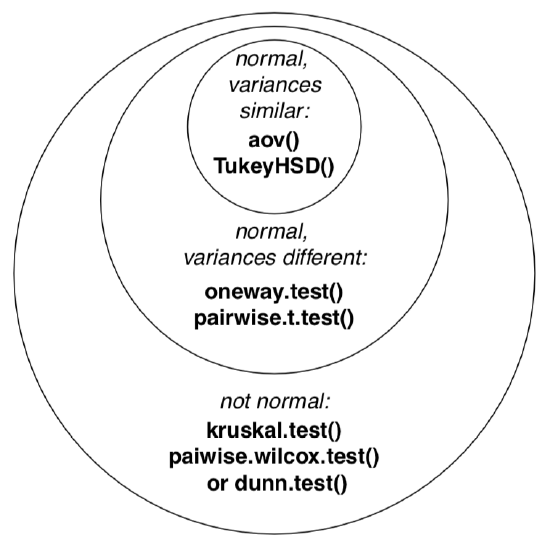
Next figure (Figure \(\PageIndex{3}\)) contains the Euler diagram which summarizes what was said above about different assumptions and ways of simple ANOVA-like analyses. Please note that there are much more post hoc tests procedures then listed, and many of them are implemented in various R packages.

The typical sequence of procedures related with one-way analysis is listed below:

• Check if data structure is suitable (head(), str(), summary()), is it long or short

• Plot (e.g., boxplot(), beanplot())

• Normality, with plot or Normality()-like function

• Homogeneity of variance (homoscedasticity) (with bartlett.test() or fligner.test())

• Core procedure (classic aov(), oneway.test() or kruskal.test())

• Optionally, effect size (\(\eta^2\) or \(\epsilon^2\) with appropriate formula)

• Post hoc test, for example TukeyHSD(), pairwise.t.test(), dunn.test() or pairwise.wilcox.test()

Figure \(\PageIndex{3}\) Applicability of different ANOVA-like procedures and related post hoc. tests. Please read it from bottom to the top.

In the open repository, data file melampyrum.txt contains results of cow-wheat (Melampyrum spp.) measurements in multiple localities. Please find if there is a difference in plant height and leaf length between plants from different localities. Which localities are divergent in each case? To understand the structure of data, use companion file melampyrum_c.txt.

All in all, if you have two or more samples represented with measurement data, the following table will help to research differences:

More then one way

Simple, one-way ANOVA uses only one factor in formula. Frequently, however, we need to analyze results of more sophisticated experiments or observations, when data is split two or more times and possibly by different principles.

Our book is not intended to go deeper, and the following is just an introduction to the world of design and analysis of experiment. Some terms, however, are important to explain:

	two samples	more then two samples
Step 1. Graphic	boxplot(); beanplot()
Step 2. Normality etc.	Normality(); hist(); qqnorm() and qqine(); optionally: bartlett. test() or flingner.test()
Step 3. Test	t.test(); wilcoxon.test()	aov(); oneway.test(); kruskal.test()
Step 4. Effect	cohen.d(); cliff.delta()	optionally: Eta2(); Epsilon2()
Step 5. Pairwise	NA	TukeyHSD(); pairwise.t.test(); dunn.test()

Table \(\PageIndex{1}\) How to research differences between numerical samples in R.

Two-way

This is when data contains two independent factors. See, for example, ?ToothGrowth data embedded in R. With more factors, three- and more ways layouts are possible.

Repeated measurements

This is analogous to paired two-sample cases, but with three and more measurements on each subject. This type of layout might require specific approaches. See ?Orange or ?Loblolly data.

Unbalanced

When groups have different sizes and/or some factor combinations are absent, then design is unbalanced; this sometimes complicates calculations.

Interaction

If there are more than one factor, they could work together (interact) to produce response. Consequently, with two factors, analysis should include statistics for each of them plus separate statistic for interaction, three values in total. We will return to interaction later, in section about ANCOVA (“Many lines”). Here we only mention the useful way to show interactions visually, with interaction plot (Figure \(\PageIndex{4}\)):

Code \(\PageIndex{24}\) (R):

with(ToothGrowth, interaction.plot(supp, dose, len))

(It is, for example, easy to see from this interaction plot that with dose 2, type of supplement does not matter.)

Random and fixed effects

Some factors are irrelevant to the research but participate in response, therefore they must be included into analysis. Other factors are planned and intentional.

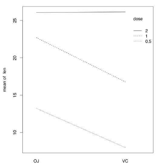
Figure \(\PageIndex{4}\) Interaction plot for ToothGrowth data.

Respectively, they are called random and fixed effects. This difference also influences calculations.

References

1. Bennett C.M., Wolford G.L., Miller M.B. 2009. The principled control of false positives in neuroimag- ing. Social cognitive and affective neuroscience 4(4): 417–422, https://www.ncbi.nlm.nih.gov/ pmc/articles/PMC2799957/

2. Like it is implemented in the ARTool package; there also possible to use multi-way nonparametric designs.