4.4: Normality

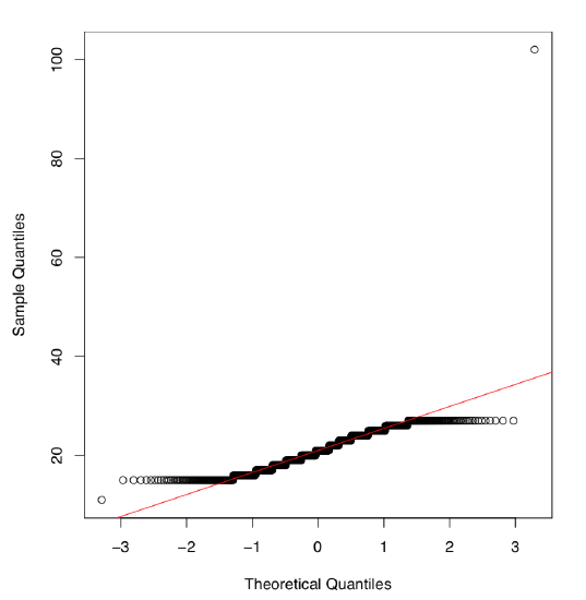
How to decide which test to use, parametric or non-parametric, t-test or Wilcoxon? We need to know if the distribution follows or at least approaches normality. This could be checked visually (Figure \(\PageIndex{1}\)):

Code \(\PageIndex{1}\) (R):

salary <- c(21, 19, 27, 11, 102, 25, 21)
new.1000 <- sample((median(salary) - IQR(salary)) : + (median(salary) + IQR(salary)), 1000, replace=TRUE)
salary2 <- c(salary, new.1000)
qqnorm(salary2, main=""); qqline(salary2, col=2)

How does QQ plot work? First, data points are ordered and each one is assigned to a quantile. Second, a set of theoretical quantiles—positions that data points should have occupied in a normal distribution—is calculated. Finally, theoretical and empirical quantiles are paired off and plotted.

We have overlaid the plot with a line coming through quartiles. When the dots follow the line closely, the empirical distribution is normal. Here a lot of dots at the tails are far. Again, we conclude, that the original distribution is not normal.

R also offers numerical instruments that check for normality. The first among them is Shapiro-Wilk test (please run this code yourself):

Code \(\PageIndex{2}\) (R):

salary <- c(21, 19, 27, 11, 102, 25, 21)
new.1000 <- sample((median(salary) - IQR(salary)) : + (median(salary) + IQR(salary)), 1000, replace=TRUE)
salary2 <- c(salary, new.1000)
shapiro.test(salary)
shapiro.test(salary2)

Here the output is rather terse. P-values are small, but what was the null hypothesis? Even the built-in help does not state it. To understand, we may run a simple experiment:

Code \(\PageIndex{3}\) (R):

set.seed(1638) # freeze random number generator
shapiro.test(rnorm(100))

The command rnorm() generates random numbers that follow normal distribution, as many of them as stated in the argument. Here we have obtained a p-value approaching unity. Clearly, the null hypothesis was “the empirical distribution is normal”.

Figure \(\PageIndex{1}\) Graphical check for the normality.

Armed with this little experiment, we may conclude that distributions of both salary and salary2 are not normal.

Kolmogorov-Smirnov test works with two distributions. The null hypothesis is that both samples came from the same population. If we want to test one distribution against normal, second argument should be pnorm:

Code \(\PageIndex{4}\) (R):

salary <- c(21, 19, 27, 11, 102, 25, 21)
new.1000 <- sample((median(salary) - IQR(salary)) : + (median(salary) + IQR(salary)), 1000, replace=TRUE)
salary2 <- c(salary, new.1000)
ks.test(scale(salary2), "pnorm")

(The result is comparable with the result of Shapiro-Wilk test. We scaled data because by default, the second argument uses scaled normal distribution.)

Function ks.test() accepts any type of the second argument and therefore could be used to check how reliable is to approximate current distribution with any theoretical distribution, not necessarily normal. However, Kolmogorov-Smirnov test often returns the wrong answer for samples which size is \(< 50\), so it is less powerful then Shapiro-Wilks test.

2.2e-16 us so-called exponential notation, the way to show really small numbers like this one (\(2.2 \times 10^{-16}\)). If this notation is not comfortable to you, there is a way to get rid of it:

Code \(\PageIndex{5}\) (R):

salary <- c(21, 19, 27, 11, 102, 25, 21)
new.1000 <- sample((median(salary) - IQR(salary)) : + (median(salary) + IQR(salary)), 1000, replace=TRUE)
salary2 <- c(salary, new.1000)
old.options <- options(scipen=100)
ks.test(scale(salary2), "pnorm")
options(old.options)

(Option scipen equals to the maximal allowable number of zeros.)

Most of times these three ways to determine normality are in agreement, but this is not a surprise if they return different results. Normality check is not a death sentence, it is just an opinion based on probability.

Again, if sample size is small, statistical tests and even quantile-quantile plots frequently fail to detect non-normality. In these cases, simpler tools like stem plot or histogram, would provide a better help.