3.3: Colors, Names and Sexes - Nominal Data

Nominal, or categorical, data, unlike ranked, are impossible to order or align. They are even farther away from numbers. For example, if we assign numerical values to males and females (say, “1” and “2”), it would not imply that one sex is somehow “larger” then the other. An intermediate value (like “1.5”) is also hard to imagine. Consequently, nominal indices may be labeled with any letters, words or special characters—it does not matter.

Regular numerical methods are just not applicable to nominal data. There are, however, ways around. The simplest one is counting, calculating frequencies for each level of nominal variable. These counts, and other derived measures, are easier to analyze.

Character vectors

R has several ways to store nominal data. First is a character (textual) vector:

Code \(\PageIndex{1}\) (R):

sex <- c("male", "female", "male", "male", "female", "male", "male")
is.character(sex)
is.vector(sex)
str(sex)

(Please note the function str() again. It is must be used each time when you deal with new objects!)

By the way, to enter character strings manually, it is easier to start with something like aa <- c(""""), then insert commas and spaces: aa <- c("", "") and finally insert values: aa <- c("b", "c").

Another option is to enter scan(what="char") and then type characters without quotes and commas; at the end, enter empty string.

Let us suppose that vector sex records sexes of employees in a small firm. This is how R displays its content:

Code \(\PageIndex{2}\) (R):

sex <- c("male", "female", "male", "male", "female", "male", "male")
sex

To select elements from the vector, use square brackets:

Code \(\PageIndex{3}\) (R):

sex <- c("male", "female", "male", "male", "female", "male", "male")
sex[2:3]

Yes, square brackets are the command! They are used to index vectors and other R objects. To prove it, run ?"[". Another way to check that is with backticks which allow to use non-trivial calls which are illegal otherwise:

Code \(\PageIndex{4}\) (R):

sex <- c("male", "female", "male", "male", "female", "male", "male")
`[`(sex, 2:3)

Smart, object-oriented functions in R may “understand” something about object sex:

Code \(\PageIndex{5}\) (R):

sex <- c("male", "female", "male", "male", "female", "male", "male")
table(sex)

Command table() counts items of each type and outputs the table, which is one of few numerical ways to work with nominal data (next section tells more about counts).

Factors

But plot() could do nothing with the character vector (check it yourself). To plot the nominal data, we are to inform R first that this vector has to be treated as factor:

Code \(\PageIndex{6}\) (R):

sex <- c("male", "female", "male", "male", "female", "male", "male")
sex.f <- factor(sex)
sex.f

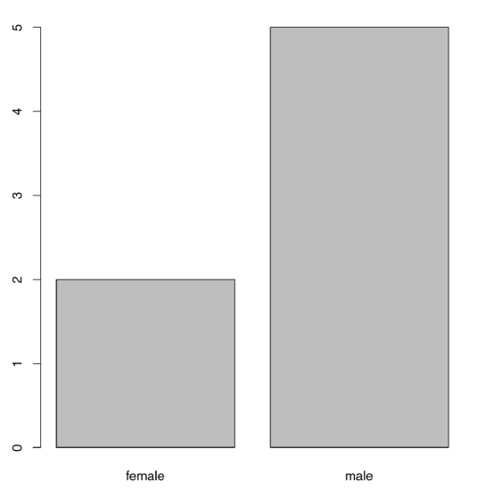
Now plot() will “see” what to do. It will invisibly count items and draw a barplot (Figure \(\PageIndex{1}\)):

Code \(\PageIndex{7}\) (R):

sex <- c("male", "female", "male", "male", "female", "male", "male")
sex.f <- factor(sex)
plot(sex.f)

It happened because character vector was transformed into an object of a type specific to categorical data, a factor with two levels:

Code \(\PageIndex{8}\) (R):

sex <- c("male", "female", "male", "male", "female", "male", "male")
sex.f <- factor(sex)
is.factor(sex.f)
is.character(sex.f)
str(sex.f)
levels(sex.f)

Figure \(\PageIndex{1}\) This is how plot() plots a factor.

Code \(\PageIndex{9}\) (R):

sex <- c("male", "female", "male", "male", "female", "male", "male")
sex.f <- factor(sex)
nlevels(sex.f)

In R, many functions (including plot()) prefer factors to character vectors. Some of them could even transform character into factor, but some not. Therefore, be careful!

There are some other facts to keep in mind.

First (and most important), factors, unlike character vectors, allow for easy transformation into numbers:

Code \(\PageIndex{10}\) (R):

sex <- c("male", "female", "male", "male", "female", "male", "male")
sex.f <- factor(sex)
as.numeric(sex.f)

But why is female 1 and male 2? Answer is really simple: because “female” is the first in alphabetical order. R uses this order every time when factors have to be converted into numbers.

Reasons for such transformation become transparent in a following example. Suppose, we also measured weights of the employees from a previous example:

Code \(\PageIndex{11}\) (R):

w <- c(69, 68, 93, 87, 59, 82, 72)

We may wish to plot all three variables: height, weight and sex. Here is one possible way (Figure \(\PageIndex{2}\)):

Code \(\PageIndex{12}\) (R):

x <- c(174, 162, 188, 192, 165, 168, 172.5)
sex <- c("male", "female", "male", "male", "female", "male", "male")
sex.f <- factor(sex)
w <- c(69, 68, 93, 87, 59, 82, 72)
plot(x, w, pch=as.numeric(sex.f), col=as.numeric(sex.f), xlab="Height, cm", ylab="Weight, kg")
legend("topleft", pch=1:2, col=1:2, legend=levels(sex.f))

Figure \(\PageIndex{2}\) A plot with three variables.

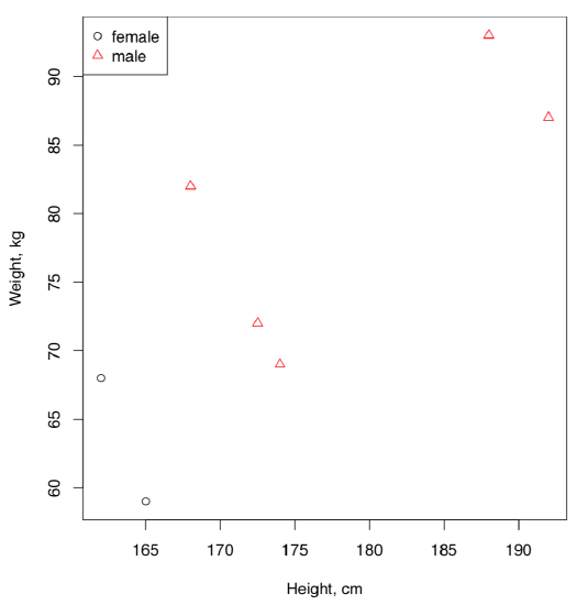
Parameters pch (from “print character”) and col (from “color”) define shape and color of the characters displayed in the plot. Depending on the value of the variable sex, data point is displayed as a circle or triangle, and also in black or in red. In general, it is enough to use either shape, or color to distinguish between levels.

Note that colors were printed from numbers in accordance with the current palette. To see which numbers mean which colors, type:

Code \(\PageIndex{13}\) (R):

palette()

It is possible to change the default palette using this function with argument. For example, palette(rainbow(8)) will replace default with 8 new “rainbow” colors. To return, type palette("default"). It is also possible to create your own palette, for example with function colorRampPalette() (see examples in next chapters) or using the separate package (like RColorBrewer or cetcolor, the last allows to create perceptually uniform palettes).

How to color barplot from Figure \(\PageIndex{1}\) in black (female) and red (male)?

If your factor is made from numbers and you want to convert it back into numbers (this task is not rare!), convert it first to the characters vector, and only then—to numbers:

Code \(\PageIndex{14}\) (R):

(ff <- factor(3:5))
as.numeric(ff) # incorrect!
as.numeric(as.character(ff)) # correct!

Next important feature of factors is that subset of a factor retains by default the original number of levels, even if some of the levels are not here anymore. Compare:

Code \(\PageIndex{15}\) (R):

sex <- c("male", "female", "male", "male", "female", "male", "male")
sex.f <- factor(sex)
sex.f[5:6]
sex.f[6:7]

There are several ways to exclude the unused levels, e.g. with droplevels() command, with drop argument, or by “back and forth” (factor to character to factor) transformation of the data:

Code \(\PageIndex{16}\) (R):

sex <- c("male", "female", "male", "male", "female", "male", "male")
sex.f <- factor(sex)
droplevels(sex.f[6:7])
sex.f[6:7, drop=T]
factor(as.character(sex.f[6:7]))

Third, we may order factors. Let us introduce a fourth variable—T-shirt sizes for these seven hypothetical employees:

Code \(\PageIndex{17}\) (R):

m <- c("L", "S", "XL", "XXL", "S", "M", "L")
m.f <- factor(m)
m.f

Here levels follow alphabetical order, which is not appropriate because we want S (small) to be the first. Therefore, we must tell R that these data are ordered:

Code \(\PageIndex{18}\) (R):

m <- c("L", "S", "XL", "XXL", "S", "M", "L")
m.f <- factor(m)
m.o <- ordered(m.f, levels=c("S", "M", "L", "XL", "XXL"))
m.o

(Now R recognizes relationships between sizes, and m.o variable could be treated as ranked.)

In this section, we created quite a few new R objects. One of skills to develop is to understand which objects are present in your session at the moment. To see them, you might want to list objects:

Code \(\PageIndex{19}\) (R):

ls()

If you want all objects together with their structure, use ls.str() command.

There is also a more sophisticated version of object listing, which reports objects in a table:

Code \(\PageIndex{20}\) (R):

Ls() # asmisc.r

(To use Ls(), either download asmisc.r and then source() it from the disk, or source from URL mentioned in the preface.)

Ls() is also handy when you start to work with large objects: it helps to clean R memory\(^{[1]}\).

Logical vectors and binary data

Binary data (do not mix with a binary file format) are a special case related with both nominal and ranked data. A good example would be “yes” of “no” reply in a questionnaire, or presence vs. absence of something. Sometimes, binary data may be ordered (as with presence/absence), sometimes not (as with right or wrong answers). Binary data may be presented either as 0/1 numbers, or as logical vector which is the string of TRUE or FALSE values.

Imagine that we asked seven employees if they like pizza and encoded their “yes”/“no” answers into TRUE or FALSE:

Code \(\PageIndex{21}\) (R):

(likes.pizza <- c(T, T, F, F, T, T, F))

Resulted vector is not character or factor, it is logical. One of interesting features is that logical vectors participate in arithmetical operations without problems. It is also easy to convert them into numbers directly with as.numeric(), as well as to convert numbers into logical with as.logical():

Code \(\PageIndex{22}\) (R):

(likes.pizza <- c(T, T, F, F, T, T, F))
is.vector(likes.pizza)
is.factor(likes.pizza)
is.character(likes.pizza)
is.logical(likes.pizza)
likes.pizza * 1
as.logical(c(1, 1, 0))
as.numeric(likes.pizza)

This is the most useful feature of binary data. All other types of data, from measurement to nominal (the last is most useful), could be converted into logical, and logical is easy to convert into 0/1 numbers:

Code \(\PageIndex{23}\) (R):

sex <- c("male", "female", "male", "male", "female", "male", "male")
Tobin(sex, convert.names=FALSE)

Afterwards, many specialized methods, such as logistic regression or binary similarity metrics, will become available even to that initially nominal data.

As an example, this is how to convert the character sex vector into logical:

Code \(\PageIndex{24}\) (R):

sex <- c("male", "female", "male", "male", "female", "male", "male")
(is.male <- sex == "male")
(is.female <- sex == "female")

(We applied logical expression on the right side of assignment using “is equal?” double equation symbol operator. This is the second numerical way to work with nominal data. Note that one character vector with two types of values became two logical vectors.)

Logical vectors are useful also for indexing:

Code \(\PageIndex{25}\) (R):

x <- c(174, 162, 188, 192, 165, 168, 172.5)
x > 170
x[x > 170]

(First, we applied logical expression with greater sign to create the logical vector. Second, we used square brackets to index heights vector; in other words, we selected those heights which are greater than 170 cm.)

Apart from greater and equal signs, there are many other logical operators which allow to create logical expressions in R(see Table \(\PageIndex{1}\)):

==	EQUAL
<=	EQUAL OR LESS
>=	EQUAL OR MORE
&	AND
|	OR
!	NOT
!=	NOT EQUAL
%in%	MATCH

Table \(\PageIndex{1}\) Some logical operators and how to understand them.

AND and OR operators (& and |) help to build truly advanced and highly useful logical expressions:

Code \(\PageIndex{26}\) (R):

x <- c(174, 162, 188, 192, 165, 168, 172.5)
sex <- c("male", "female", "male", "male", "female", "male", "male")
w <- c(69, 68, 93, 87, 59, 82, 72)
((x < 180) | (w <= 70)) & (sex=="female" | m=="S")

(Here we selected only those people which height is less than 170 cm or weight is 70 kg or less, these people must also be either females or bear small size T-shirts. Note that use of parentheses allows to control the order of calculations and also makes expression more understandable.)

Logical expressions are even more powerful if you learn how to use them together with command ifelse() and operator if (the last is frequently supplied with else):

Code \(\PageIndex{27}\) (R):

sex <- c("male", "female", "male", "male", "female", "male", "male")
ifelse(sex=="female", "pink", "blue")

(Command ifelse() is vectorized so it goes through multiple conditions at once. Operator if takes only one condition.)

Note the use of curly braces it the last rows. Curly braces turn a number of expressions into a single (combined) expression. When there is only a single command, the curly braces are optional. Curly braces may contain two commands on one row if they are separated with semicolon.

References

1. By default, Ls() does not output functions. If required, this behavior could be changed withLs(exclude="none").