26.1: Linear Regression

We can also use the general linear model to describe the relation between two variables and to decide whether that relationship is statistically significant; in addition, the model allows us to predict the value of the dependent variable given some new value(s) of the independent variable(s). Most importantly, the general linear model will allow us to build models that incorporate multiple independent variables, whereas correlation can only tell us about the relationship between two individual variables.

The specific version of the GLM that we use for this is referred to as as linear regression. The term regression was coined by Francis Galton, who had noted that when he compared parents and their children on some feature (such as height), the children of extreme parents (i.e. the very tall or very short parents) generally fell closer to the mean than their parents. This is an extremely important point that we return to below.

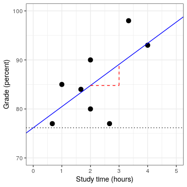
The simplest version of the linear regression model (with a single independent variable) can be expressed as follows:

$$y = x * \beta_x + \beta_0 + \epsilon$$ The $\beta_x$ value tells us how much we would expect y to change given a one-unit change in x. The intercept $\beta_0$ is an overall offset, which tells us what value we would expect y to have when $x=0$; you may remember from our early modeling discussion that this is important to model the overall magnitude of the data, even if $x$ never actually attains a value of zero. The error term $\epsilon$ refers to whatever is left over once the model has been fit. If we want to know how to predict y (which we call $\hat{y}$), then we can drop the error term:

$$\hat{y}=x*{\beta }_x+{\beta }_0$$

Figure 26.2: The linear regression solution for the study time data is shown in the solid line The value of the intercept is equivalent to the predicted value of the y variable when the x variable is equal to zero; this is shown with a dotted line. The value of beta is equal to the slope of the line – that is, how much y changes for a unit change in x. This is shown schematically in the dashed lines, which show the degree of increase in grade for a single unit increase in study time.

We will not go into the details of how the best fitting slope and intercept are actually estimated from the data; if you are interested, details are available in the Appendix.

26.1.1 Regression to the mean

The concept of regression to the mean was one of Galton’s essential contributions to science, and it remains a critical point to understand when we interpret the results of experimental data analyses. Let’s say that we want to study the effects of a reading intervention on the performance of poor readers. To test our hypothesis, we might go into a school and recruit those individuals in the bottom 25% of the distribution on some reading test, administer the intervention, and then examine their performance. Let’s say that the intervention actually has no effect, such that reading scores for each individual are simply independent samples from a normal distribution. We can simulate this:

Table 26.1: Reading scores for Test 1 (which is lower, because it was the basis for selecting the students) and Test 2 (which is higher because it was not related to Test 1).

	Score
Test 1	88
Test 2	101

If we look at the difference between the mean test performance at the first and second test, it appears that the intervention has helped these students substantially, as their scores have gone up by more than ten points on the test! However, we know that in fact the students didn’t improve at all, since in both cases the scores were simply selected from a random normal distribution. What has happened is that some subjects scored badly on the first test simply due to random chance. If we select just those subjects on the basis of their first test scores, they are guaranteed to move back towards the mean of the entire group on the second test, even if there is no effect of training. This is the reason that we need an untreated control group in order to interpret any changes in reading over time; otherwise we are likely to be tricked by regression to the mean.

26.1.2 The relation between correlation and regression

There is a close relationship between correlation coefficients and regression coefficients. Remember that Pearson’s correlation coefficient is computed as the ratio of the covariance and the product of the standard deviations of x and y:

$$\hat{r} = \frac{covariance_{xy}}{s_x * s_y}$$ whereas the regression beta is computed as:

$$\hat{\beta} = \frac{covariance_{xy}}{s_x*s_x}$$

Based on these two equations, we can derive the relationship between $\hat{r}$ and $\hat{beta}$:

$$covariance_{xy} = \hat{r} * s_x * s_y$$

$$\hat{\beta_x} = \frac{\hat{r} * s_x * s_y}{s_x * s_x} = r * \frac{s_y}{s_x}$$ That is, the regression slope is equal to the correlation value multiplied by the ratio of standard deviations of y and x. One thing this tells us is that when the standard deviations of x and y are the same (e.g. when the data have been converted to Z scores), then the correlation estimate is equal to the regression slope estimate.

26.1.3 Standard errors for regression models

If we want to make inferences about the regression parameter estimates, then we also need an estimate of their variability. To compute this, we first need to compute the residual variance or error variance for the model – that is, how much variability in the dependent variable is not explained by the model. We can compute the model residuals as follows:

$$residual = y - \hat{y} = y - (x*\hat{\beta_x} + \hat{\beta_0})$$ We then compute the sum of squared errors (SSE):

$$SS_{error} = \sum_{i=1}^n{(y_i - \hat{y_i})^2} = \sum_{i=1}^n{residuals^2}$$ and from this we compute the mean squared error:

$$MS_{error} = \frac{SS_{error}}{df} = \frac{\sum_{i=1}^n{(y_i - \hat{y_i})^2} }{N - p}$$ where the degrees of freedom ($df$) are determined by subtracting the number of estimated parameters (2 in this case: $\hat{\beta_x}$ and $\hat{\beta_0}$) from the number of observations ($N$). Once we have the mean squared error, we can compute the standard error for the model as:

$$SE_{model} = \sqrt{MS_{error}}$$

In order to get the standard error for a specific regression parameter estimate, $SE$, we need to rescale the standard error of the model by the square root of the sum of squares of the X variable:

$$SE_{\beta_x} = \frac{SE_{model}}{\sqrt$$

ParseError: invalid DekiScript (click for details)

Callstack:
    at (Bookshelves/Introductory_Statistics/Statistical_Thinking_for_the_21st_Century_(Poldrack)/26:_The_General_Linear_Model/26.01:_Linear_Regression), /content/body/section[3]/div/p[7]/math/semantics/annotation/span, line 1, column 1

}

26.1.4 Statistical tests for regression parameters

Once we have the parameter estimates and their standard errors, we can compute a t statistic to tell us the likelihood of the observed parameter estimates compared to some expected value under the null hypothesis. In this case we will test against the null hypothesis of no effect (i.e. $\beta=0$):

$$\begin{array}{c} t_{N - p} = \frac{\hat{\beta} - \beta_{expected}}{SE_{\hat{\beta}}}\\ t_{N - p} = \frac{\hat{\beta} - 0}{SE_{\hat{\beta}}}\\ t_{N - p} = \frac{\hat{\beta} }{SE_{\hat{\beta}}} \end{array}$$

In R, we don’t need to compute these by hand, as they are automatically returned to us by the lm() function:

## 
## Call:
## lm(formula = grade ~ studyTime, data = df)
## 
## Residuals:
##     Min      1Q  Median      3Q     Max 
## -10.656  -2.719   0.125   4.703   7.469 
## 
## Coefficients:
##             Estimate Std. Error t value Pr(>|t|)    
## (Intercept)    76.16       5.16   14.76  6.1e-06 ***
## studyTime       4.31       2.14    2.01    0.091 .  
## ---
## Signif. codes:  0 '***' 0.001 '**' 0.01 '*' 0.05 '.' 0.1 ' ' 1
## 
## Residual standard error: 6.4 on 6 degrees of freedom
## Multiple R-squared:  0.403,  Adjusted R-squared:  0.304 
## F-statistic: 4.05 on 1 and 6 DF,  p-value: 0.0907

In this case we see that the intercept is significantly different from zero (which is not very interesting) and that the effect of studyTime on grades is marginally significant (p = .09).

26.1.5 Quantifying goodness of fit of the model

Sometimes it’s useful to quantify how well the model fits the data overall, and one way to do this is to ask how much of the variability in the data is accounted for by the model. This is quantified using a value called $R$ (also known as the coefficient of determination). If there is only one x variable, then this is easy to compute by simply squaring the correlation coefficient:

$$R^2 = r^2$$ In the case of our study time example, $R$ = 0.4, which means that we have accounted for about 40% of the variance in grades.

More generally we can think of $R$ as a measure of the fraction of variance in the data that is accounted for by the model, which can be computed by breaking the variance into multiple components:

$$SS_{total} = SS_{model} + SS_{error}$$ where $SS$ is the variance of the data ($y$) and $SS$ and $SS$ are computed as shown earlier in this chapter. Using this, we can then compute the coefficient of determination as:

$$R^2 = \frac{SS_{model}}{SS_{total}} = 1 - \frac{SS_{error}}{SS_{total}}$$

A small value of $R$ tells us that even if the model fit is statistically significant, it may only explain a small amount of information in the data.