
24.3: Covariance and Correlation
- Page ID
- 8843

One way to quantify the relationship between two variables is the covariance. Remember that variance for a single variable is computed as the average squared difference between each data point and the mean:
This tells us how far each observation is from the mean, on average, in squared units. Covariance tells us whether there is a relation between the deviations of two different variables across observations. It is defined as:
This value will be far from zero when x and y are both highly deviant from the mean; if they are deviant in the same direction then the covariance is positive, whereas if they are deviant in opposite directions the covariance is negative. Let’s look at a toy example first. The data are shown in the table, along with their individual deviations from the mean and their crossproducts.
| x | y | y_dev | x_dev | crossproduct |
|---|---|---|---|---|
| 3 | 5 | -3.6 | -4.6 | 16.56 |
| 5 | 4 | -4.6 | -2.6 | 11.96 |
| 8 | 7 | -1.6 | 0.4 | -0.64 |
| 10 | 10 | 1.4 | 2.4 | 3.36 |
| 12 | 17 | 8.4 | 4.4 | 36.96 |
The covariance is simply the mean of the crossproducts, which in this case is 17.05. We don’t usually use the covariance to describe relationships between variables, because it varies with the overall level of variance in the data. Instead, we would usually use the correlation coefficient (often referred to as Pearson’s correlation after the statistician Karl Pearson). The correlation is computed by scaling the covariance by the standard deviations of the two variables:
In this case, the value is0.89. We can also compute the correlation value easily using the cor() function in R, rather than computing it by hand.
The correlation coefficient is useful because it varies between -1 and 1 regardless of the nature of the data - in fact, we already discussed the correlation coefficient earlier in the discussion of effect sizes. As we saw in the previous chapter on effect sizes, a correlation of 1 indicates a perfect linear relationship, a correlation of -1 indicates a perfect negative relationship, and a correlation of zero indicates no linear relationship.
24.3.1 Hypothesis testing for correlations
The correlation value of 0.42 seems to indicate a reasonably strong relationship between the hate crimes and income inequality, but we can also imagine that this could occur by chance even if there is no relationship. We can test the null hypothesis that the correlation is zero, using a simple equation that lets us convert a correlation value into a t statistic:
\(t_{r}=\frac{r \sqrt{N-2}}{\sqrt{1-r^{2}}}\)
Under the null hypothesis , this statistic is distributed as a t distribution with degrees of freedom. We can compute this using the cor.test() function in R:
##
##  Pearson's product-moment correlation
##
## data:  hateCrimes$avg_hatecrimes_per_100k_fbi and hateCrimes$gini_index
## t = 3, df = 48, p-value = 0.002
## alternative hypothesis: true correlation is not equal to 0
## 95 percent confidence interval:
##  0.16 0.63
## sample estimates:
##  cor
## 0.42
This test shows that the likelihood of an r value this extreme or more is quite low, so we would reject the null hypothesis of . Note that this test assumes that both variables are normally distributed.
We could also test this by randomization, in which we repeatedly shuffle the values of one of the variables and compute the correlation, and then compare our observed correlation value to this null distribution to determine how likely our observed value would be under the null hypothesis. The results are shown in Figure 24.2. The p-value computed using randomization is reasonably similar to the answer give by the t-test.
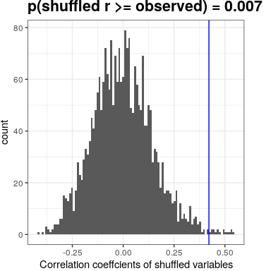
Figure 24.2: Histogram of correlation values under the null hypothesis, obtained by shuffling values. Observed value is denoted by blue line.
We could also use Bayesian inference to estimate the correlation; see the Appendix for more on this.
24.3.2 Robust correlations
You may have noticed something a bit odd in Figure 24.1 – one of the datapoints (the one for the District of Columbia) seemed to be quite separate from the others. We refer to this as an outlier, and the standard correlation coefficient is very sensitive to outliers. For example, in Figure 24.3 we can see how a single outlying data point can cause a very high positive correlation value, even when the actual relationship between the other data points is perfectly negative.
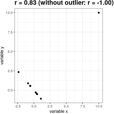
Figure 24.3: An simulated example of the effects of outliers on correlation. Without the outlier the remainder of the datapoints have a perfect negative correlation, but the single outlier changes the correlation value to highly positive.
One way to address outliers is to compute the correlation on the ranks of the data after ordering them, rather than on the data themselves; this is known as the Spearman correlation. Whereas the Pearson correlation for the example in Figure 24.3 was 0.83, the Spearman correlation is -0.45, showing that the rank correlation reduces the effect of the outlier.
We can compute the rank correlation on the hate crime data using the cor.test function:
##
##  Spearman's rank correlation rho
##
## data:  hateCrimes$avg_hatecrimes_per_100k_fbi and hateCrimes$gini_index
## S = 20146, p-value = 0.8
## alternative hypothesis: true rho is not equal to 0
## sample estimates:
##   rho
## 0.033
Now we see that the correlation is no longer significant (and in fact is very near zero), suggesting that the claims of the FiveThirtyEight blog post may have been incorrect due to the effect of the outlier.