14.5: Using Simulation for Statistics- The Bootstrap

So far we have used simulation to demonstrate statistical principles, but we can also use simulation to answer real statistical questions. In this section we will introduce a concept known as the bootstrap that lets us use simulation to quantify our uncertainty about statistical estimates. Later in the course, we will see other examples of how simulation can often be used to answer statistical questions, especially when theoretical statistical methods are not available or when their assumptions are too difficult to meet.

14.5.1 Computing the bootstrap

In the section above, we used our knowledge of the sampling distribution of the mean to compute the standard error of the mean and confidence intervals. But what if we can’t assume that the estimates are normally distributed, or we don’t know their distribution? The idea of the bootstrap is to use the data themselves to estimate an answer. The name comes from the idea of pulling one’s self up by one’s own bootstraps, expressing the idea that we don’t have any external source of leverage so we have to rely upon the data themselves. The bootstrap method was conceived by Bradley Efron of the Stanford Department of Statistics, who is one of the world’s most influential statisticians.

The idea behind the bootstrap is that we repeatedly sample from the actual dataset; importantly, we sample with replacement, such that the same data point will often end up being represented multiple times within one of the samples. We then compute our statistic of interest on each of the bootstrap samples, and use the distribution of those estimates.

Let’s start by using the bootstrap to estimate the sampling distribution of the mean, so that we can compare the result to the standard error of the mean (SEM) that we discussed earlier.

Figure 14.4: An example of bootstrapping to compute the standard error of the mean. The histogram shows the distribution of means across bootstrap samples, while the red line shows the normal distribution based on the sample mean and standard deviation.

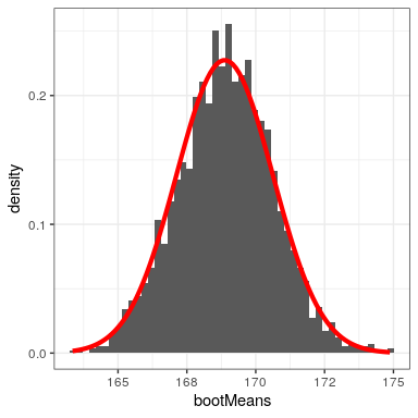
Figure 14.4 shows that the distribution of means across bootstrap samples is fairly close to the theoretical estimate based on the assumption of normality. We can also use the bootstrap samples to compute a confidence interval for the mean, simply by computing the quantiles of interest from the distribution of bootstrap samples.

Table 14.1: Confidence limits for normal distribution and bootstrap methods

type	2.5%	97.5%
Normal	165	172
Bootstrap	165	172

We would not usually employ the bootstrap to compute confidence intervals for the mean (since we can generally assume that the normal distribution is appropriate for the sampling distribution of the mean, as long as our sample is large enough), but this example shows how the method gives us roughly the same result as the standard method based on the normal distribution. The bootstrap would more often be used to generate standard errors for estimates of other statistics where we know or suspect that the normal distribution is not appropriate.