8.10: Z-scores

Having characterized a distribution in terms of its central tendency and variability, it is often useful to express the individual scores in terms of where they sit with respect to the overall distribution. Let’s say that we are interested in characterizing the relative level of crimes across different states, in order to determine whether California is a particularly dangerous place. We can ask this question using data for 2014 from the FBI’s Uniform Crime Reporting site. The left panel of Figure 8.8 shows a histogram of the number of violent crimes per state, highlighting the value for California. Looking at these data, it seems like California is terribly dangerous, with 153709 crimes in that year.

Figure 8.8: Left: Histogram of the number of violent crimes. The value for CA is plotted in blue. Right: A map of the same data, with number of crimes plotted for each state in color.

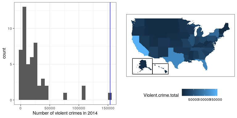
With R it’s also easy to generate a map showing the distribution of a variable across states, which is presented in the right panel of Figure 8.8.

It may have occurred to you, however, that CA also has the largest population of any state in the US, so it’s reasonable that it will also have a larger number of crimes. If we plot the two against one another (see left panel of Figure 8.9), we see that there is a direct relationship between population and the number of crimes.

Figure 8.9: Left: A plot of number of crimes versus population by state. Right: A histogram of per capita crime rates, expressed as crimes per 100,000 people.

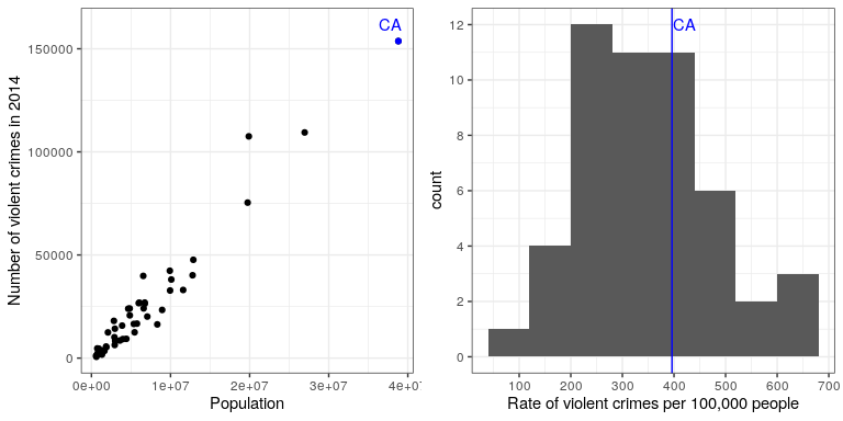
Instead of using the raw numbers of crimes, we should instead use the per-capita violent crime rate, which we obtain by dividing the number of crimes by the population of the state. The dataset from the FBI already includes this value (expressed as rate per 100,000 people). Looking at the right panel of Figure 8.9, we see that California is not so dangerous after all – its crime rate of 396.10 per 100,000 people is a bit above the mean across states of 346.81, but well within the range of many other states. But what if we want to get a clearer view of how far it is from the rest of the distribution?

The Z-score allows us to express data in a way that provides more insight into each data point’s relationship to the overall distribution. The formula to compute a Z-score for a data point given that we know the value of the population mean $\mu$ and standard deviation $\sigma$ is:

$$Z(x)=\frac{x-\mu }{\sigma }$$

Intuitively, you can think of a Z-score as telling you how far away from the mean any data point is, in units of standard deviation. We can compute this for the crime rate data, as shown in Figure 8.10.

## [1] "mean of Z-scored data: 1.4658413372004e-16"

## [1] "std deviation of Z-scored data: 1"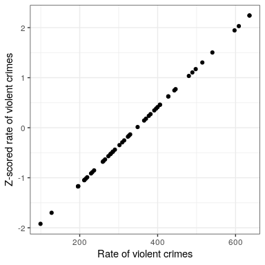

Figure 8.10: Scatterplot of original crime rate data against Z-scored data.

The scatterplot shows us that the process of Z-scoring doesn’t change the relative distribution of the data points (visible in the fact that the orginal data and Z-scored data fall on a straight line when plotted against each other) – it just shifts them to have a mean of zero and a standard deviation of one. However, if you look closely, you will see that the mean isn’t exactly zero – it’s just very small. What is going on here is that the computer represents numbers with a certain amount of numerical precision - which means that there are numbers that are not exactly zero, but are small enough that R considers them to be zero.

Figure 8.11 shows the Z-scored crime data using the geographical view.

Figure 8.11: Crime data rendered onto a US map, presented as Z-scores.

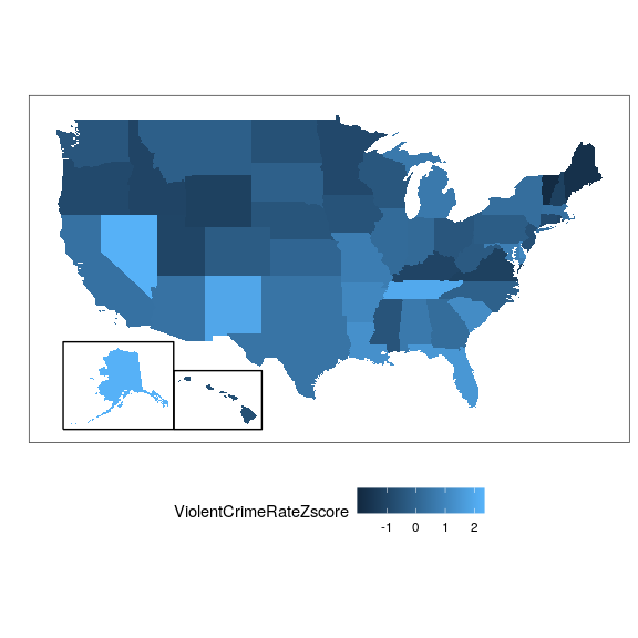
This provides us with a slightly more interpretable view of the data. For example, we can see that Nevada, Tennessee, and New Mexico all have crime rates that are roughly two standard deviations above the mean.

8.9.1 Interpreting Z-scores

The “Z” in “Z-score”" comes from the fact that the standard normal distribution (that is, a normal distribution with a mean of zero and a standard deviation of 1) is often referred to as the “Z” distribution. We can use the standard normal distribution to help us understand what specific Z scores tell us about where a data point sits with respect to the rest of the distribution.

Figure 8.12: Density (top) and cumulative distribution (bottom) of a standard normal distribution, with cutoffs at one standard deviation above/below the mean.

The upper panel in Figure 8.12 shows that we expect about 16% of values to fall in $Z\ge 1$, and the same proportion to fall in $Z\le -1$.

Figure 8.13: Density (top) and cumulative distribution (bottom) of a standard normal distribution, with cutoffs at two standard deviations above/below the mean

Figure 8.13 shows the same plot for two standard deviations. Here we see that only about 2.3% of values fall in $Z \le -2$ and the same in $Z \ge 2$. Thus, if we know the Z-score for a particular data point, we can estimate how likely or unlikely we would be to find a value at least as extreme as that value, which lets us put values into better context.

8.9.2 Standardized scores

Let’s say that instead of Z-scores, we wanted to generate standardized crime scores with a mean of 100 and standard deviation of 10. This is similar to the standardization that is done with scores from intelligence tests to generate the intelligence quotient (IQ). We can do this by simply multiplying the Z-scores by 10 and then adding 100.

Figure 8.14: Crime data presented as standardized scores with mean of 100 and standard deviation of 10.

8.9.2.1 Using Z-scores to compare distributions

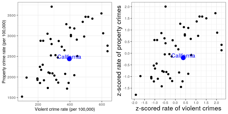
One useful application of Z-scores is to compare distributions of different variables. Let’s say that we want to compare the distributions of violent crimes and property crimes across states. In the left panel of Figure 8.15 we plot those against one another, with CA plotted in blue. As you can see the raw rates of property crimes are far higher than the raw rates of violent crimes, so we can’t just compare the numbers directly. However, we can plot the Z-scores for these data against one another (right panel of Figure 8.15)– here again we see that the distribution of the data does not change. Having put the data into Z-scores for each variable makes them comparable, and lets us see that California is actually right in the middle of the distribution in terms of both violent crime and property crime.

Figure 8.15: Plot of violent vs. property crime rates (left) and Z-scored rates (right).

Let’s add one more factor to the plot: Population. In the left panel of Figure 8.16 we show this using the size of the plotting symbol, which is often a useful way to add information to a plot.

Figure 8.16: Left: Plot of violent vs. property crime rates, with population size presented through the size of the plotting symbol; California is presented in blue. Right: Difference scores for violent vs. property crime, plotted against population.

Because Z-scores are directly comparable, we can also compute a “Violence difference” score that expresses the relative rate of violent to non-violent (property) crimes across states. We can then plot those scores against population (see right panel of Figure 8.16). This shows how we can use Z-scores to bring different variables together on a common scale.

It is worth noting that the smallest states appear to have the largest differences in both directions. While it might be tempting to look at each state and try to determine why it has a high or low difference score, this probably reflects the fact that the estimates obtained from smaller samples are necessarily going to be more variable, as we will discuss in the later chapter on Sampling.