
2.4: Relative Position of Data
- Page ID
- 558
- To learn the concept of the relative position of an element of a data set.
- To learn the meaning of each of two measures, the percentile rank and the \(z\)-score, of the relative position of a measurement and how to compute each one.
- To learn the meaning of the three quartiles associated to a data set and how to compute them.
- To learn the meaning of the five-number summary of a data set, how to construct the box plot associated to it, and how to interpret the box plot.
When you take an exam, what is often as important as your actual score on the exam is the way your score compares to other students’ performance. If you made a \(70\) but the average score (whether the mean, median, or mode) was \(85\), you did relatively poorly. If you made a \(70\) but the average score was only \(55\) then you did relatively well. In general, the significance of one observed value in a data set strongly depends on how that value compares to the other observed values in a data set. Therefore we wish to attach to each observed value a number that measures its relative position.
Percentiles and Quartiles
Anyone who has taken a national standardized test is familiar with the idea of being given both a score on the exam and a “percentile ranking” of that score. You may be told that your score was \(625\) and that it is the \(85^{th}\) percentile. The first number tells how you actually did on the exam; the second says that \(85\%\) of the scores on the exam were less than or equal to your score, \(625\).
Given an observed value \(x\) in a data set, \(x\) is the \(P^{th}\) percentile of the data if \(P\%\) of the data are less than or equal to \(x\). The number \(P\) is the percentile rank of \(x\).
Example \(\PageIndex{1}\)
What percentile is the value \(1.39\) in the data set of ten GPAs considered in a previous Example? What percentile is the value \(3.33\)?
Solution
The data, written in increasing order, are
\[ \begin{array}{cccccccccc} 1.39 & 1.76 & 1.90 & 2.12 & 2.53 & 2.71 & 3.00 & 3.33 & 3.71 & 4.00 \end{array} \nonumber \]
The only data value that is less than or equal to \(1.39\) is \(1.39\) itself. Since \(1\) out of ten, or \(1/10=10\%\), of the data points are less than or equal to \(1.39\), \(1.39\) is the \(10^{th}\) percentile. Eight data values are less than or equal to \(3.33\). Since \(8\) out of ten, or \(8∕10 = .80 = 80\%\) of the data values are less than or equal to \(3.33\), the value \(3.33\) is the \(80^{th}\) percentile of the data.
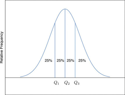
The Pth percentile cuts the data set in two so that approximately \(P\%\) of the data lie below it and \((100−P)\% \) of the data lie above it. In particular, the three percentiles that cut the data into fourths, as shown in Figure \(\PageIndex{1}\), are called the quartiles of a data set. The quartiles are the three numbers \(Q_1\), \(Q_2\), \(Q_3\) that divide the data set approximately into fourths. The following simple computational definition of the three quartiles works well in practice.
Definition: quartile
For any data set:
- The second quartile \(Q_2\) of the data set is its median.
- Define two subsets:
- the lower set: all observations that are strictly less than \(Q_2\)
- the upper set: all observations that are strictly greater than \(Q_2\)
- The first quartile \(Q_1\) of the data set is the median of the lower set.
- The third quartile \(Q_3\) of the data set is the median of the upper set.
Example \(\PageIndex{2}\)
Find the quartiles of the data set of GPAs of discussed in a previous Example.
Solution
As in the previous example we first list the data in numerical order:
\[\begin{array}{cccccccccc} 1.39 & 1.76 & 1.90 & 2.12 & 2.53 & 2.71 & 3.00 & 3.33 & 3.71 & 4.00 \end{array} \nonumber \]
This data set has \(n=10\) observations. Since \(10\) is an even number, the median is the mean of the two middle observations:
\[\tilde x=(2.53+2.71)∕2=2.62. \nonumber \]
Thus the second quartile is \(Q_2=2.62\). The lower and upper subsets are
- Lower: \(L=\{1.39,1.76,1.90,2.12,2.53\}\),
- Upper: \(U=\{2.71,3.00,3.33,3.71,4.00\}\).
Each has an odd number of elements, so the median of each is its middle observation. Thus the first quartile is \(Q_1=1.90\), the median of \(L\), and the third quartile is \(Q_3=3.33\), the median of \(U\).
Example \(\PageIndex{3}\)
Adjoin the observation \(3.88\) to the data set of the previous example and find the quartiles of the new set of data.
Solution
As in the previous example we first list the data in numerical order:
\[\begin{array}{ccccccccccc} 1.39 & 1.76 & 1.90 & 2.12 & 2.53 & 2.71 & 3.00 & 3.33 & 3.71 & 3.88, 4.00 \end{array} \nonumber \]
This data set has \(11\) observations. The second quartile is its median, the middle value \(2.71\). Thus \(Q_2=2.71\). The lower and upper subsets are now
- Lower: \(L=\{1.39,1.76,1.90,2.12,2.53\}\)
- Upper: \(U=\{3.00,3.33,3.71,3.88,4.00\}\).
The lower set \(L\) has median, the middle value, \(1.90\), so \(Q_1=1.90\). The upper set has median \(3.71\), so \(Q_3=3.71\).
In addition to the three quartiles, the two extreme values, the minimum \(x_{min}\) and the maximum \(x_{max}\) are also useful in describing the entire data set. Together these five numbers are called the five-number summary of a data set,
{ \(X_{min}\), \(Q_1\), \(Q_2\), \(Q_3\), \(X_{max}\) }
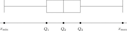
The five-number summary is used to construct a box plot, as in Figure \(\PageIndex{2}\). Each of the five numbers is represented by a vertical line segment, a box is formed using the line segments at \(Q_1\) and \(Q_3\) as its two vertical sides, and two horizontal line segments are extended from the vertical segments marking \(Q_1\) and \(Q_3\) to the adjacent extreme values. (The two horizontal line segments are referred to as “whiskers,” and the diagram is sometimes called a "box and whisker plot.") We caution the reader that there are other types of box plots that differ somewhat from the ones we are constructing, although all are based on the three quartiles.
Note that the distance from \(Q1\) to \(Q3\) is the length of the interval over which the middle half of the data range. Thus it has the following special name.
The interquartile range \(IQR\) is the quantity
\[IQR = Q3-Q1 \nonumber \]
Example \(\PageIndex{4}\)
Construct a box plot and find the \(IQR\) for the data in Example \(\PageIndex{3}\).
Solution
From our work in Example \(\PageIndex{1}\), we know that the five-number summary is
- \(X_{min} = 1.39\)
- \(Q1 = 1.90\)
- \(Q2 = 2.62\)
- \(Q3 = 3.33\)
- \(X_{max} = 4.00\)
The box plot is:
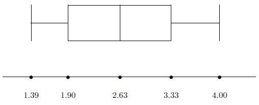
The interquartile range is: \(IQR=3.33-1.90=1.43\).
\(z\)-Scores
Another way to locate a particular observation \(x\) in a data set is to compute its distance from the mean in units of standard deviation. The \(z\)-score indicates how many standard deviations an individual observation \(x\) is from the center of the data set, its mean. It is used on distributions that have been standardized, which allows us to better understand its properties. If \(z\) is negative then \(x\) is below average. If \(z\) is \(0\) then \(x\) is equal to the average. If \(z\) is positive then \(x\) is above the average
Definition: \(z\)-score
The \(z\)-score of an observation \(x\) is the number \(z\) given by the computational formula
\[z = \dfrac{x - \mu}{\sigma} \nonumber \]
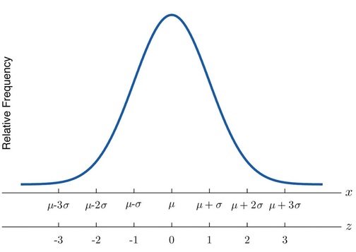
Figure \(\PageIndex{3}\): x-Scale versus z-Score
Suppose the mean and standard deviation of the GPA's of all currently registered students at a college are \(\mu = 2.70\) and \(\sigma = 0.50\). The \(z\)-scores of the GPA's of two students, Antonio and Beatrice, are \(z=-0.62\) and \(z=1.28\), respectively. What are their GPAs?
Solution
Using the second formula right after the definition of \(z\)-scores we compute the GPA's as
- Antonio: \(x=\mu +z\sigma =2.70+(-0.62)(0.50)=2.39\)
- Beatrice: \(x=\mu +z\sigma =2.70+(1.28)(0.50)=3.34\)
Key Takeaways
- The percentile rank and \(z\)-score of a measurement indicate its relative position with regard to the other measurements in a data set.
- The three quartiles divide a data set into fourths.
- The five-number summary and its associated box plot summarize the location and distribution of the data.