
2.3: Measures of Variability
- Page ID
- 557
- To learn the concept of the variability of a data set.
- To learn how to compute three measures of the variability of a data set: the range, the variance, and the standard deviation.
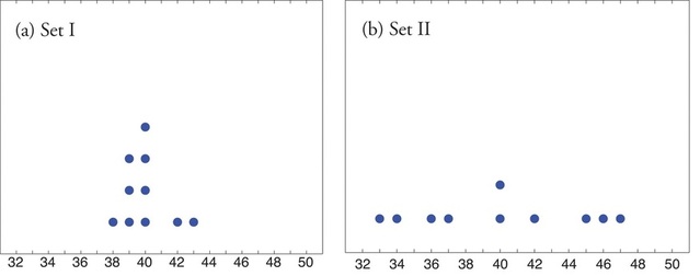
Look at the two data sets in Table \(\PageIndex{1}\) and the graphical representation of each, called a dot plot, in Figure \(\PageIndex{1}\).
| Data Set I: | 40 | 38 | 42 | 40 | 39 | 39 | 43 | 40 | 39 | 40 |
|---|---|---|---|---|---|---|---|---|---|---|
| Data Set II: | 46 | 37 | 40 | 33 | 42 | 36 | 40 | 47 | 34 | 45 |
The two sets of ten measurements each center at the same value: they both have mean, median, and mode \(40\). Nevertheless a glance at the figure shows that they are markedly different. In Data Set I the measurements vary only slightly from the center, while for Data Set II the measurements vary greatly. Just as we have attached numbers to a data set to locate its center, we now wish to associate to each data set numbers that measure quantitatively how the data either scatter away from the center or cluster close to it. These new quantities are called measures of variability, and we will discuss three of them.
The Range
First we discuss the simplest measure of variability.
The range \(R\) of a data set is difference between its largest and smallest values \[R=x_{\text{max}}−x_{\text{min}} \nonumber \] where \(\displaystyle x_{\text{max}}\) is the largest measurement in the data set and \(\displaystyle x_{\text{min}}\) is the smallest.
Find the range of each data set in Table \(\PageIndex{1}\).
Solution
- For Data Set I the maximum is \(43\) and the minimum is \(38\), so the range is \(R=43−38=5\).
- For Data Set II the maximum is \(47\) and the minimum is \(33\), so the range is \(R=47−33=14\).
The range is a measure of variability because it indicates the size of the interval over which the data points are distributed. A smaller range indicates less variability (less dispersion) among the data, whereas a larger range indicates the opposite.
The Variance and the Standard Deviation
The other two measures of variability that we will consider are more elaborate and also depend on whether the data set is just a sample drawn from a much larger population or is the whole population itself (that is, a census).
The sample variance of a set of \(n\) sample data is the number \(\mathbf{ s^2}\) defined by the formula
\[s^2 = \dfrac{\sum (x-\bar x)^2}{n-1} \nonumber \]
which by algebra is equivalent to the formula
\[s^2=\dfrac{\sum x^2 - \dfrac{1}{n}\left(\sum x\right)^2}{n-1} \nonumber \]
The square root \(\mathbf s\) of the sample variance is called the sample standard deviation of a set of \(n\) sample data . It is given by the formulas
\[s = \sqrt{s^2} = \sqrt{\dfrac{\sum (x-\bar x)^2}{n-1} } = \sqrt{\dfrac{\sum x^2 - \dfrac{1}{n}\left(\sum x\right)^2}{n-1}}. \nonumber \]
Although the first formula in each case looks less complicated than the second, the latter is easier to use in hand computations, and is called a shortcut formula.
Find the sample variance and the sample standard deviation of Data Set II in Table \(\PageIndex{1}\).
Solution
To use the defining formula (the first formula) in the definition we first compute for each observation \(x\) its deviation \(x-\bar x\) from the sample mean. Since the mean of the data is \(\bar x =40\), we obtain the ten numbers displayed in the second line of the supplied table
\[ \begin{array}{c|cccccccccc} x & 46 & 37 & 40 & 33 & 42 & 36 & 40 & 47 & 34 & 45 \\ \hline x−\bar{x} & -6 & -3 & 0 & -7 & 2 & -4 & 0 & 7 & -6 & 5 \end{array} \nonumber \]
Thus
\[\sum (x-\bar{x})^2=6^2+(-3)^2+0^2+(-7)^2+2^2+(-4)^2+0^2+7^2+(-6)^2+5^2=224\nonumber \]
so the variance is
\[s^2=\dfrac{\sum (x-\bar{x})^2}{n-1}=\dfrac{224}{9}=24.\bar{8} \nonumber \]
and the standard deviation is
\[s=\sqrt{24.\bar{8}} \approx 4.99 \nonumber \]
The student is encouraged to compute the ten deviations for Data Set I and verify that their squares add up to \(20\), so that the sample variance and standard deviation of Data Set I are the much smaller numbers
\[s^2=20/9=2.\bar{2} \nonumber \]
and
\[s=20/9 \approx 1.49 \nonumber \]
Find the sample variance and the sample standard deviation of the ten GPAs in "Example 2.2.3" in Section 2.2.
\[1.90\; \; 3.00\; \; 2.53\; \; 3.71\; \; 2.12\; \; 1.76\; \; 2.71\; \; 1.39\; \; 4.00\; \; 3.33\nonumber \]
Solution
Since
\[ \sum x = 1.90 + 3.00+ 2.53 + 3.71 + 2.12 + 1.76 + 2.71 + 1.39 + 4.00 + 3.33 = 26.45 \nonumber \]
and
\[ \sum x^2 = 1.902 + 3.002 + 2.532 + 3.712 + 2.122+ 1.762 + 2.712 + 1.392 + 4.002 + 3.332 = 76.7321 \nonumber \]
the shortcut formula gives
\[ s^2=\dfrac{\sum x^2−(\sum x)^2}{n−1}=\dfrac{76.7321−(26.45)^2/10}{10−1}=\dfrac{6.77185}{9}=0.75242\bar{7} \nonumber \]
and
\[ s=\sqrt{0.75242\bar{7}}\approx 0.867 \nonumber \]
The sample variance has different units from the data. For example, if the units in the data set were inches, the new units would be inches squared, or square inches. It is thus primarily of theoretical importance and will not be considered further in this text, except in passing.
If the data set comprises the whole population, then the population standard deviation, denoted \(\sigma\) (the lower case Greek letter sigma), and its square, the population variance \(\sigma ^2\), are defined as follows.
The variability of a set of \(N\) population data is measured by the population variance
\[\sigma^2=\dfrac{\sum (x−\mu)^2}{N} \label{popVar} \]
and its square root, the population standard deviation
\[\sigma =\sqrt{\dfrac{\sum (x−\mu)^2}{N}}\label{popSTD} \]
where \(\mu\) is the population mean as defined above.
Note that the denominator in the fraction is the full number of observations, not that number reduced by one, as is the case with the sample standard deviation. Since most data sets are samples, we will always work with the sample standard deviation and variance.
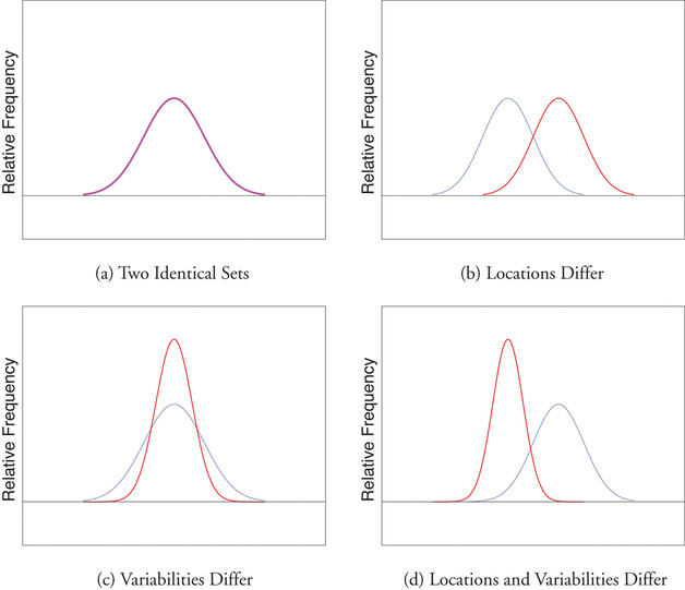
Finally, in many real-life situations the most important statistical issues have to do with comparing the means and standard deviations of two data sets. Figure \(\PageIndex{2}\) illustrates how a difference in one or both of the sample mean and the sample standard deviation are reflected in the appearance of the data set as shown by the curves derived from the relative frequency histograms built using the data.
Key Takeaway
The range, the standard deviation, and the variance each give a quantitative answer to the question “How variable are the data?”