
10.2: Two Population Means with Unknown Standard Deviations
- Page ID
- 778

- The two independent samples are simple random samples from two distinct populations.
- For the two distinct populations:
- if the sample sizes are small, the distributions are important (should be normal)
- if the sample sizes are large, the distributions are not important (need not be normal)
The test comparing two independent population means with unknown and possibly unequal population standard deviations is called the Aspin-Welch \(t\)-test. The degrees of freedom formula was developed by Aspin-Welch.
The comparison of two population means is very common. A difference between the two samples depends on both the means and the standard deviations. Very different means can occur by chance if there is great variation among the individual samples. In order to account for the variation, we take the difference of the sample means, \(\bar{X}_{1} - \bar{X}_{2}\), and divide by the standard error in order to standardize the difference. The result is a t-score test statistic.
Because we do not know the population standard deviations, we estimate them using the two sample standard deviations from our independent samples. For the hypothesis test, we calculate the estimated standard deviation, or standard error, of the difference in sample means, \(\bar{X}_{1} - \bar{X}_{2}\).
The standard error is:
\[\sqrt{\dfrac{(s_{1})^{2}}{n_{1}} + \dfrac{(s_{2})^{2}}{n_{2}}}\]
The test statistic (t-score) is calculated as follows:
\[\dfrac{(\bar{x}-\bar{x}) - (\mu_{1} - \mu_{2})}{\sqrt{\dfrac{(s_{1})^{2}}{n_{1}} + \dfrac{(s_{2})^{2}}{n_{2}}}}\]
where:
- \(s_{1}\) and \(s_{2}\), the sample standard deviations, are estimates of \(\sigma_{1}\) and \(\sigma_{1}\), respectively.
- \(\sigma_{1}\) and \(\sigma_{2}\) are the unknown population standard deviations.
- \(\bar{x}_{1}\) and \(\bar{x}_{2}\) are the sample means. \(\mu_{1}\) and \(\mu_{2}\) are the population means.
The number of degrees of freedom (\(df\)) requires a somewhat complicated calculation. However, a computer or calculator calculates it easily. The \(df\) are not always a whole number. The test statistic calculated previously is approximated by the Student's t-distribution with \(df\) as follows:
\[df = \dfrac{\left(\dfrac{(s_{1})^{2}}{n_{1}} + \dfrac{(s_{2})^{2}}{n_{2}}\right)^{2}}{\left(\dfrac{1}{n_{1}-1}\right)\left(\dfrac{(s_{1})^{2}}{n_{1}}\right)^{2} + \left(\dfrac{1}{n_{2}-1}\right)\left(\dfrac{(s_{2})^{2}}{n_{2}}\right)^{2}}\]
When both sample sizes \(n_{1}\) and \(n_{2}\) are five or larger, the Student's t approximation is very good. Notice that the sample variances \((s_{1})^{2}\) and \((s_{2})^{2}\) are not pooled. (If the question comes up, do not pool the variances.)
It is not necessary to compute the degrees of freedom by hand. A calculator or computer easily computes it.
The average amount of time boys and girls aged seven to 11 spend playing sports each day is believed to be the same. A study is done and data are collected, resulting in the data in Table \(\PageIndex{1}\). Each populations has a normal distribution.
| Sample Size | Average Number of Hours Playing Sports Per Day | Sample Standard Deviation | |
|---|---|---|---|
| Girls | 9 | 2 | 0.8660.866 |
| Boys | 16 | 3.2 | 1.00 |
Is there a difference in the mean amount of time boys and girls aged seven to 11 play sports each day? Test at the 5% level of significance.
Answer
The population standard deviations are not known. Let g be the subscript for girls and b be the subscript for boys. Then, \(\mu_{g}\) is the population mean for girls and \(\mu_{b}\) is the population mean for boys. This is a test of two independent groups, two population means.
Random variable: \(\bar{X}_{g} - \bar{X}_{b} =\) difference in the sample mean amount of time girls and boys play sports each day.
- \(H_{0}: \mu_{g} = \mu_{b}\)
- \(H_{0}: \mu_{g} - \mu_{b} = 0\)
- \(H_{a}: \mu_{g} \neq \mu_{b}\)
- \(H_{a}: \mu_{g} - \mu_{b} \neq 0\)
The words "the same" tell you \(H_{0}\) has an "=". Since there are no other words to indicate \(H_{a}\), assume it says "is different." This is a two-tailed test.
Distribution for the test: Use \(t_{df}\) where \(df\) is calculated using the \(df\) formula for independent groups, two population means. Using a calculator, \(df\) is approximately 18.8462. Do not pool the variances.
Calculate the p-value using a Student's t-distribution: \(p\text{-value} = 0.0054\)
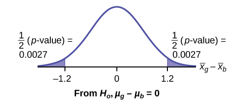
Graph:
\[s_{g} = 0.866\]
\[s_{b} = 1\]
So,
\[\bar{x}_{g} - \bar{x}_{b} = 2 - 3.2 = -1.2\]
Half the \(p\text{-value}\) is below –1.2 and half is above 1.2.
Make a decision: Since \(\alpha > p\text{-value}\), reject \(H_{0}\). This means you reject \(\mu_{g} = \mu_{b}\). The means are different.
Press STAT. Arrow over to TESTS and press 4:2-SampTTest. Arrow over to Stats and press ENTER. Arrow down and enter 2 for the first sample mean, \(\sqrt{0.866}\) for Sx1, 9 for n1, 3.2 for the second sample mean, 1 for Sx2, and 16 for n2. Arrow down to μ1: and arrow to does not equal μ2. Press ENTER. Arrow down to Pooled: and No. Press ENTER. Arrow down to Calculate and press ENTER. The \(p\text{-value}\) is \(p = 0.0054\), the dfs are approximately 18.8462, and the test statistic is -3.14. Do the procedure again but instead of Calculate do Draw.
Conclusion: At the 5% level of significance, the sample data show there is sufficient evidence to conclude that the mean number of hours that girls and boys aged seven to 11 play sports per day is different (mean number of hours boys aged seven to 11 play sports per day is greater than the mean number of hours played by girls OR the mean number of hours girls aged seven to 11 play sports per day is greater than the mean number of hours played by boys).
Two samples are shown in Table. Both have normal distributions. The means for the two populations are thought to be the same. Is there a difference in the means? Test at the 5% level of significance.
| Sample Size | Sample Mean | Sample Standard Deviation | |
|---|---|---|---|
| Population A | 25 | 5 | 1 |
| Population B | 16 | 4.7 | 1.2 |
Answer
The \(p\text{-value}\) is \(0.4125\), which is much higher than 0.05, so we decline to reject the null hypothesis. There is not sufficient evidence to conclude that the means of the two populations are not the same.
When the sum of the sample sizes is larger than \(30 (n_{1} + n_{2} > 30)\) you can use the normal distribution to approximate the Student's \(t\).
A study is done by a community group in two neighboring colleges to determine which one graduates students with more math classes. College A samples 11 graduates. Their average is four math classes with a standard deviation of 1.5 math classes. College B samples nine graduates. Their average is 3.5 math classes with a standard deviation of one math class. The community group believes that a student who graduates from college A has taken more math classes, on the average. Both populations have a normal distribution. Test at a 1% significance level. Answer the following questions.
- Is this a test of two means or two proportions?
- Are the populations standard deviations known or unknown?
- Which distribution do you use to perform the test?
- What is the random variable?
- What are the null and alternate hypotheses? Write the null and alternate hypotheses in words and in symbols.
- Is this test right-, left-, or two-tailed?
- What is the \(p\text{-value}\)?
- Do you reject or not reject the null hypothesis?
Solutions
- two means
- unknown
- Student's t
- \(\bar{X}_{A} - \bar{X}_{B}\)
- \(H_{0}: \mu_{A} \leq \mu_{B}\) and \(H_{a}: \mu_{A} > \mu_{B}\)
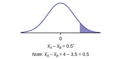
right
- g. 0.1928
- h. Do not reject.
- i. At the 1% level of significance, from the sample data, there is not sufficient evidence to conclude that a student who graduates from college A has taken more math classes, on the average, than a student who graduates from college B.
A study is done to determine if Company A retains its workers longer than Company B. Company A samples 15 workers, and their average time with the company is five years with a standard deviation of 1.2. Company B samples 20 workers, and their average time with the company is 4.5 years with a standard deviation of 0.8. The populations are normally distributed.
- Are the population standard deviations known?
- Conduct an appropriate hypothesis test. At the 5% significance level, what is your conclusion?
Answer
- They are unknown.
- The \(p\text{-value} = 0.0878\). At the 5% level of significance, there is insufficient evidence to conclude that the workers of Company A stay longer with the company.
A professor at a large community college wanted to determine whether there is a difference in the means of final exam scores between students who took his statistics course online and the students who took his face-to-face statistics class. He believed that the mean of the final exam scores for the online class would be lower than that of the face-to-face class. Was the professor correct? The randomly selected 30 final exam scores from each group are listed in Table \(\PageIndex{3}\) and Table \(\PageIndex{4}\).
| 67.6 | 41.2 | 85.3 | 55.9 | 82.4 | 91.2 | 73.5 | 94.1 | 64.7 | 64.7 |
| 70.6 | 38.2 | 61.8 | 88.2 | 70.6 | 58.8 | 91.2 | 73.5 | 82.4 | 35.5 |
| 94.1 | 88.2 | 64.7 | 55.9 | 88.2 | 97.1 | 85.3 | 61.8 | 79.4 | 79.4 |
| 77.9 | 95.3 | 81.2 | 74.1 | 98.8 | 88.2 | 85.9 | 92.9 | 87.1 | 88.2 |
| 69.4 | 57.6 | 69.4 | 67.1 | 97.6 | 85.9 | 88.2 | 91.8 | 78.8 | 71.8 |
| 98.8 | 61.2 | 92.9 | 90.6 | 97.6 | 100 | 95.3 | 83.5 | 92.9 | 89.4 |
Is the mean of the Final Exam scores of the online class lower than the mean of the Final Exam scores of the face-to-face class? Test at a 5% significance level. Answer the following questions:
- Is this a test of two means or two proportions?
- Are the population standard deviations known or unknown?
- Which distribution do you use to perform the test?
- What is the random variable?
- What are the null and alternative hypotheses? Write the null and alternative hypotheses in words and in symbols.
- Is this test right, left, or two tailed?
- What is the \(p\text{-value}\)?
- Do you reject or not reject the null hypothesis?
- At the ___ level of significance, from the sample data, there ______ (is/is not) sufficient evidence to conclude that ______.
(See the conclusion in Example, and write yours in a similar fashion)
Be careful not to mix up the information for Group 1 and Group 2!
Answer
- two means
- unknown
- Student's \(t\)
- \(\bar{X}_{1} - \bar{X}_{2}\)
-
- \(H_{0}: \mu_{1} = \mu_{2}\) Null hypothesis: the means of the final exam scores are equal for the online and face-to-face statistics classes.
- \(H_{a}: \mu_{1} < \mu_{2}\) Alternative hypothesis: the mean of the final exam scores of the online class is less than the mean of the final exam scores of the face-to-face class.
- left-tailed
- \(p\text{-value} = 0.0011\)
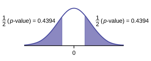
Figure \(\PageIndex{3}\).
- Reject the null hypothesis
- The professor was correct. The evidence shows that the mean of the final exam scores for the online class is lower than that of the face-to-face class.
At the 5% level of significance, from the sample data, there is (is/is not) sufficient evidence to conclude that the mean of the final exam scores for the online class is less than the mean of final exam scores of the face-to-face class.
First put the data for each group into two lists (such as L1 and L2). Press STAT. Arrow over to TESTS and press 4:2SampTTest. Make sure Data is highlighted and press ENTER. Arrow down and enter L1 for the first list and L2 for the second list. Arrow down to \(\mu_{1}\): and arrow to \(\neq \mu_{1}\) (does not equal). Press ENTER. Arrow down to Pooled: No. Press ENTER. Arrow down to Calculate and press ENTER.
Cohen's Standards for Small, Medium, and Large Effect Sizes
Cohen's \(d\) is a measure of effect size based on the differences between two means. Cohen’s \(d\), named for United States statistician Jacob Cohen, measures the relative strength of the differences between the means of two populations based on sample data. The calculated value of effect size is then compared to Cohen’s standards of small, medium, and large effect sizes.
| Size of effect | \(d\) |
|---|---|
| Small | 0.2 |
| medium | 0.5 |
| Large | 0.8 |
Cohen's \(d\) is the measure of the difference between two means divided by the pooled standard deviation: \(d = \dfrac{\bar{x}_{2}-\bar{x}_{2}}{s_{\text{pooled}}}\) where \(s_{pooled} = \sqrt{\dfrac{(n_{1}-1)s^{2}_{1} + (n_{2}-1)s^{2}_{2}}{n_{1}+n_{2}-2}}\)
Calculate Cohen’s d for Example. Is the size of the effect small, medium, or large? Explain what the size of the effect means for this problem.
Answer
\(\mu_{1} = 4 s_{1} = 1.5 n_{1} = 11\)
\(\mu_{2} = 3.5 s_{2} = 1 n_{2} = 9\)
\(d = 0.384\)
The effect is small because 0.384 is between Cohen’s value of 0.2 for small effect size and 0.5 for medium effect size. The size of the differences of the means for the two colleges is small indicating that there is not a significant difference between them.
Calculate Cohen’s \(d\) for Example. Is the size of the effect small, medium or large? Explain what the size of the effect means for this problem.
Answer
\(d = 0.834\); Large, because 0.834 is greater than Cohen’s 0.8 for a large effect size. The size of the differences between the means of the Final Exam scores of online students and students in a face-to-face class is large indicating a significant difference.
Weighted alpha is a measure of risk-adjusted performance of stocks over a period of a year. A high positive weighted alpha signifies a stock whose price has risen while a small positive weighted alpha indicates an unchanged stock price during the time period. Weighted alpha is used to identify companies with strong upward or downward trends. The weighted alpha for the top 30 stocks of banks in the northeast and in the west as identified by Nasdaq on May 24, 2013 are listed in Table and Table, respectively.
| 94.2 | 75.2 | 69.6 | 52.0 | 48.0 | 41.9 | 36.4 | 33.4 | 31.5 | 27.6 |
| 77.3 | 71.9 | 67.5 | 50.6 | 46.2 | 38.4 | 35.2 | 33.0 | 28.7 | 26.5 |
| 76.3 | 71.7 | 56.3 | 48.7 | 43.2 | 37.6 | 33.7 | 31.8 | 28.5 | 26.0 |
| 126.0 | 70.6 | 65.2 | 51.4 | 45.5 | 37.0 | 33.0 | 29.6 | 23.7 | 22.6 |
| 116.1 | 70.6 | 58.2 | 51.2 | 43.2 | 36.0 | 31.4 | 28.7 | 23.5 | 21.6 |
| 78.2 | 68.2 | 55.6 | 50.3 | 39.0 | 34.1 | 31.0 | 25.3 | 23.4 | 21.5 |
Is there a difference in the weighted alpha of the top 30 stocks of banks in the northeast and in the west? Test at a 5% significance level. Answer the following questions:
- Is this a test of two means or two proportions?
- Are the population standard deviations known or unknown?
- Which distribution do you use to perform the test?
- What is the random variable?
- What are the null and alternative hypotheses? Write the null and alternative hypotheses in words and in symbols.
- Is this test right, left, or two tailed?
- What is the \(p\text{-value}\)?
- Do you reject or not reject the null hypothesis?
- At the ___ level of significance, from the sample data, there ______ (is/is not) sufficient evidence to conclude that ______.
- Calculate Cohen’s d and interpret it.
Answer
- two means
- unknown
- Student’s-t
- \(\bar{X}_{1} - \bar{X}_{2}\)
-
- \(H_{0}: \mu_{1} = \mu_{2}\) Null hypothesis: the means of the weighted alphas are equal.
- \(H_{a}: \mu_{1} \neq \mu_{2}\) Alternative hypothesis : the means of the weighted alphas are not equal.
- two-tailed
- \(p\text{-value} = 0.8787\)
- Do not reject the null hypothesis
- This indicates that the trends in stocks are about the same in the top 30 banks in each region.

Figure \(\PageIndex{4}\).
5% level of significance, from the sample data, there is not sufficient evidence to conclude that the mean weighted alphas for the banks in the northeast and the west are different - \(d = 0.040\), Very small, because 0.040 is less than Cohen’s value of 0.2 for small effect size. The size of the difference of the means of the weighted alphas for the two regions of banks is small indicating that there is not a significant difference between their trends in stocks.
References
- Data from Graduating Engineer + Computer Careers. Available online at www.graduatingengineer.com
- Data from Microsoft Bookshelf.
- Data from the United States Senate website, available online at www.Senate.gov (accessed June 17, 2013).
- “List of current United States Senators by Age.” Wikipedia. Available online at en.Wikipedia.org/wiki/List_of...enators_by_age (accessed June 17, 2013).
- “Sectoring by Industry Groups.” Nasdaq. Available online at www.nasdaq.com/markets/barcha...&base=industry (accessed June 17, 2013).
- “Strip Clubs: Where Prostitution and Trafficking Happen.” Prostitution Research and Education, 2013. Available online at www.prostitutionresearch.com/ProsViolPosttrauStress.html (accessed June 17, 2013).
- “World Series History.” Baseball-Almanac, 2013. Available online at http://www.baseball-almanac.com/ws/wsmenu.shtml (accessed June 17, 2013).
Review
Two population means from independent samples where the population standard deviations are not known
- Random Variable: \(\bar{X}_{1} - \bar{X}_{2} =\) the difference of the sampling means
- Distribution: Student's t-distribution with degrees of freedom (variances not pooled)
Formula Review
Standard error: \[SE = \sqrt{\dfrac{(s_{1}^{2})}{n_{1}} + \dfrac{(s_{2}^{2})}{n_{2}}}\]
Test statistic (t-score): \[t = \dfrac{(\bar{x}_{1}-\bar{x}_{2}) - (\mu_{1}-\mu_{2})}{\sqrt{\dfrac{(s_{1})^{2}}{n_{1}} + \dfrac{(s_{2})^{2}}{n_{2}}}}\]
Degrees of freedom:
\[df = \dfrac{\left(\dfrac{(s_{1})^{2}}{n_{1}} + \dfrac{(s_{2})^{2}}{n_{2}}\right)^{2}}{\left(\dfrac{1}{n_{1} - 1}\right)\left(\dfrac{(s_{1})^{2}}{n_{1}}\right)^{2}} + \left(\dfrac{1}{n_{2} - 1}\right)\left(\dfrac{(s_{2})^{2}}{n_{2}}\right)^{2}\]
where:
- \(s_{1}\) and \(s_{2}\) are the sample standard deviations, and n1 and n2 are the sample sizes.
- \(x_{1}\) and \(x_{2}\) are the sample means.
Cohen’s \(d\) is the measure of effect size:
\[d = \dfrac{\bar{x}_{1} - \bar{x}_{2}}{s_{\text{pooled}}}\]
where
\[s_{\text{pooled}} = \sqrt{\dfrac{(n_{1} - 1)s^{2}_{1} + (n_{2} - 1)s^{2}_{2}}{n_{1} + n_{2} - 2}}\]
Glossary
- Degrees of Freedom (\(df\))
- the number of objects in a sample that are free to vary.
- Standard Deviation
- A number that is equal to the square root of the variance and measures how far data values are from their mean; notation: \(s\) for sample standard deviation and \(\sigma\) for population standard deviation.
- Variable (Random Variable)
- a characteristic of interest in a population being studied. Common notation for variables are upper-case Latin letters \(X, Y, Z,\)... Common notation for a specific value from the domain (set of all possible values of a variable) are lower-case Latin letters \(x, y, z,\).... For example, if \(X\) is the number of children in a family, then \(x\) represents a specific integer 0, 1, 2, 3, .... Variables in statistics differ from variables in intermediate algebra in the two following ways.
- The domain of the random variable (RV) is not necessarily a numerical set; the domain may be expressed in words; for example, if \(X =\) hair color, then the domain is {black, blond, gray, green, orange}.
- We can tell what specific value x of the random variable \(X\) takes only after performing the experiment.