
9.5: Rare Events, the Sample, Decision and Conclusion
- Page ID
- 774

Establishing the type of distribution, sample size, and known or unknown standard deviation can help you figure out how to go about a hypothesis test. However, there are several other factors you should consider when working out a hypothesis test.
Rare Events
Suppose you make an assumption about a property of the population (this assumption is the null hypothesis). Then you gather sample data randomly. If the sample has properties that would be very unlikely to occur if the assumption is true, then you would conclude that your assumption about the population is probably incorrect. (Remember that your assumption is just an assumption—it is not a fact and it may or may not be true. But your sample data are real and the data are showing you a fact that seems to contradict your assumption.)
For example, Didi and Ali are at a birthday party of a very wealthy friend. They hurry to be first in line to grab a prize from a tall basket that they cannot see inside because they will be blindfolded. There are 200 plastic bubbles in the basket and Didi and Ali have been told that there is only one with a $100 bill. Didi is the first person to reach into the basket and pull out a bubble. Her bubble contains a $100 bill. The probability of this happening is \(\frac{1}{200} = 0.005\). Because this is so unlikely, Ali is hoping that what the two of them were told is wrong and there are more $100 bills in the basket. A "rare event" has occurred (Didi getting the $100 bill) so Ali doubts the assumption about only one $100 bill being in the basket.
Use the sample data to calculate the actual probability of getting the test result, called the \(p\)-value. The \(p\)-value is the probability that, if the null hypothesis is true, the results from another randomly selected sample will be as extreme or more extreme as the results obtained from the given sample.
A large \(p\)-value calculated from the data indicates that we should not reject the null hypothesis. The smaller the \(p\)-value, the more unlikely the outcome, and the stronger the evidence is against the null hypothesis. We would reject the null hypothesis if the evidence is strongly against it.
Draw a graph that shows the \(p\)-value. The hypothesis test is easier to perform if you use a graph because you see the problem more clearly.
Suppose a baker claims that his bread height is more than 15 cm, on average. Several of his customers do not believe him. To persuade his customers that he is right, the baker decides to do a hypothesis test. He bakes 10 loaves of bread. The mean height of the sample loaves is 17 cm. The baker knows from baking hundreds of loaves of bread that the standard deviation for the height is 0.5 cm. and the distribution of heights is normal.
- The null hypothesis could be \(H_{0}: \mu \leq 15\)
- The alternate hypothesis is \(H_{a}: \mu > 15\)
The words "is more than" translates as a "\(>\)" so "\(\mu > 15\)" goes into the alternate hypothesis. The null hypothesis must contradict the alternate hypothesis.
Since \(\sigma\) is known (\(\sigma = 0.5 cm.\)), the distribution for the population is known to be normal with mean \(μ = 15\) and standard deviation
\[\dfrac{\sigma}{\sqrt{n}} = \frac{0.5}{\sqrt{10}} = 0.16. \nonumber\]
Suppose the null hypothesis is true (the mean height of the loaves is no more than 15 cm). Then is the mean height (17 cm) calculated from the sample unexpectedly large? The hypothesis test works by asking the question how unlikely the sample mean would be if the null hypothesis were true. The graph shows how far out the sample mean is on the normal curve. The p-value is the probability that, if we were to take other samples, any other sample mean would fall at least as far out as 17 cm.
The \(p\)-value, then, is the probability that a sample mean is the same or greater than 17 cm. when the population mean is, in fact, 15 cm. We can calculate this probability using the normal distribution for means.
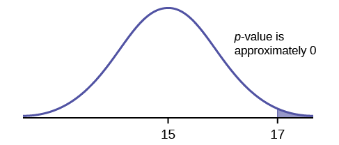
\(p\text{-value} = P(\bar{x} > 17)\) which is approximately zero.
A \(p\)-value of approximately zero tells us that it is highly unlikely that a loaf of bread rises no more than 15 cm, on average. That is, almost 0% of all loaves of bread would be at least as high as 17 cm. purely by CHANCE had the population mean height really been 15 cm. Because the outcome of 17 cm. is so unlikely (meaning it is happening NOT by chance alone), we conclude that the evidence is strongly against the null hypothesis (the mean height is at most 15 cm.). There is sufficient evidence that the true mean height for the population of the baker's loaves of bread is greater than 15 cm.
A normal distribution has a standard deviation of 1. We want to verify a claim that the mean is greater than 12. A sample of 36 is taken with a sample mean of 12.5.
- \(H_{0}: \mu \leq 12\)
- \(H_{a}: \mu > 12\)
The \(p\)-value is 0.0013
Draw a graph that shows the \(p\)-value.
- Answer
-
\(p\text{-value} = 0.0013\)
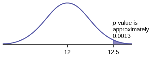
Figure \(\PageIndex{2}\)
Decision and Conclusion
A systematic way to make a decision of whether to reject or not reject the null hypothesis is to compare the \(p\)-value and a preset or preconceived \(\alpha\) (also called a "significance level"). A preset \(\alpha\) is the probability of a Type I error (rejecting the null hypothesis when the null hypothesis is true). It may or may not be given to you at the beginning of the problem.
When you make a decision to reject or not reject \(H_{0}\), do as follows:
- If \(\alpha > p\text{-value}\), reject \(H_{0}\). The results of the sample data are significant. There is sufficient evidence to conclude that \(H_{0}\) is an incorrect belief and that the alternative hypothesis, \(H_{a}\), may be correct.
- If \(\alpha \leq p\text{-value}\), do not reject \(H_{0}\). The results of the sample data are not significant.There is not sufficient evidence to conclude that the alternative hypothesis,\(H_{a}\), may be correct.
When you "do not reject \(H_{0}\)", it does not mean that you should believe that H0 is true. It simply means that the sample data have failed to provide sufficient evidence to cast serious doubt about the truthfulness of \(H_{0}\).
Conclusion: After you make your decision, write a thoughtful conclusion about the hypotheses in terms of the given problem.
When using the \(p\)-value to evaluate a hypothesis test, it is sometimes useful to use the following memory device
- If the \(p\)-value is low, the null must go.
- If the \(p\)-value is high, the null must fly.
This memory aid relates a \(p\)-value less than the established alpha (the \(p\) is low) as rejecting the null hypothesis and, likewise, relates a \(p\)-value higher than the established alpha (the \(p\) is high) as not rejecting the null hypothesis.
Fill in the blanks.
Reject the null hypothesis when ______________________________________.
The results of the sample data _____________________________________.
Do not reject the null when hypothesis when __________________________________________.
The results of the sample data ____________________________________________.
Answer
Reject the null hypothesis when the \(p\)-value is less than the established alpha value. The results of the sample data support the alternative hypothesis.
Do not reject the null hypothesis when the \(p\)-value is greater than the established alpha value. The results of the sample data do not support the alternative hypothesis.
It’s a Boy Genetics Labs claim their procedures improve the chances of a boy being born. The results for a test of a single population proportion are as follows:
- \(H_{0}: p = 0.50, H_{a}: p > 0.50\)
- \(\alpha = 0.01\)
- \(p\text{-value} = 0.025\)
Interpret the results and state a conclusion in simple, non-technical terms.
- Answer
-
Since the \(p\)-value is greater than the established alpha value (the \(p\)-value is high), we do not reject the null hypothesis. There is not enough evidence to support It’s a Boy Genetics Labs' stated claim that their procedures improve the chances of a boy being born.
Review
When the probability of an event occurring is low, and it happens, it is called a rare event. Rare events are important to consider in hypothesis testing because they can inform your willingness not to reject or to reject a null hypothesis. To test a null hypothesis, find the p-value for the sample data and graph the results. When deciding whether or not to reject the null the hypothesis, keep these two parameters in mind:
- \(\alpha > p-value\), reject the null hypothesis
- \(\alpha \leq p-value\), do not reject the null hypothesis
Glossary
- Level of Significance of the Test
- probability of a Type I error (reject the null hypothesis when it is true). Notation: \(\alpha\). In hypothesis testing, the Level of Significance is called the preconceived \(\alpha\) or the preset \(\alpha\).
- \(p\)-value
- the probability that an event will happen purely by chance assuming the null hypothesis is true. The smaller the \(p\)-value, the stronger the evidence is against the null hypothesis.