
15.3.7: Chapter 8 Lab
- Page ID
- 28621

\( \newcommand{\vecs}[1]{\overset { \scriptstyle \rightharpoonup} {\mathbf{#1}} } \) \( \newcommand{\vecd}[1]{\overset{-\!-\!\rightharpoonup}{\vphantom{a}\smash {#1}}} \)\(\newcommand{\id}{\mathrm{id}}\) \( \newcommand{\Span}{\mathrm{span}}\) \( \newcommand{\kernel}{\mathrm{null}\,}\) \( \newcommand{\range}{\mathrm{range}\,}\) \( \newcommand{\RealPart}{\mathrm{Re}}\) \( \newcommand{\ImaginaryPart}{\mathrm{Im}}\) \( \newcommand{\Argument}{\mathrm{Arg}}\) \( \newcommand{\norm}[1]{\| #1 \|}\) \( \newcommand{\inner}[2]{\langle #1, #2 \rangle}\) \( \newcommand{\Span}{\mathrm{span}}\) \(\newcommand{\id}{\mathrm{id}}\) \( \newcommand{\Span}{\mathrm{span}}\) \( \newcommand{\kernel}{\mathrm{null}\,}\) \( \newcommand{\range}{\mathrm{range}\,}\) \( \newcommand{\RealPart}{\mathrm{Re}}\) \( \newcommand{\ImaginaryPart}{\mathrm{Im}}\) \( \newcommand{\Argument}{\mathrm{Arg}}\) \( \newcommand{\norm}[1]{\| #1 \|}\) \( \newcommand{\inner}[2]{\langle #1, #2 \rangle}\) \( \newcommand{\Span}{\mathrm{span}}\)\(\newcommand{\AA}{\unicode[.8,0]{x212B}}\)
Central Limit Theorem
Open the Minitab file lab07.mpj from the website.
The lifetime of optical scanning drives follows a skewed distribution with \(\mu=100\) and \(\sigma=100\). The five columns labeled CLT \(n\)= represent 1000 simulated random samples of 1, 5, 10, 30, and 100 from this population.
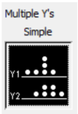
- Make dot plots of all 5 sample sizes using the Multiple Y's Simple option and paste the result here.
- As the sample size changes, describe the change in center.
- As the sample size changes, describe the change in spread.
- As the sample size changes, describe the change in shape.
- Using the command STAT>DISPLAY DESCRIPTIVE STATISTICS, determine the mean and standard deviation for each of the five groups. Paste the results here.
- The Central Limit Theorem states that the Expected Value of \(\bar{X}\) is \(\mu\). As the sample size increases, describe the change in mean. Is this consistent with the Central Limit Theorem?
- The Central Limit Theorem states that the Standard Deviation of \(\bar{X}\) is \(\sigma / \sqrt{n}\). As the sample size increases, describe the change in standard deviation. Is this consistent with the Central Limit Theorem?
- What you have observed are the three important parts of the Central Limit Theorem for the distribution of the sample mean \(\bar{X}\). In your own words, describe these three important parts.