15.2.13: Chapter 14 Homework

Last updated
Save as PDF

Page ID: 28316

\( \newcommand{\vecs}[1]{\overset { \scriptstyle \rightharpoonup} {\mathbf{#1}} } \) \( \newcommand{\vecd}[1]{\overset{-\!-\!\rightharpoonup}{\vphantom{a}\smash {#1}}} \)\(\newcommand{\id}{\mathrm{id}}\) \( \newcommand{\Span}{\mathrm{span}}\) \( \newcommand{\kernel}{\mathrm{null}\,}\) \( \newcommand{\range}{\mathrm{range}\,}\) \( \newcommand{\RealPart}{\mathrm{Re}}\) \( \newcommand{\ImaginaryPart}{\mathrm{Im}}\) \( \newcommand{\Argument}{\mathrm{Arg}}\) \( \newcommand{\norm}[1]{\| #1 \|}\) \( \newcommand{\inner}[2]{\langle #1, #2 \rangle}\) \( \newcommand{\Span}{\mathrm{span}}\) \(\newcommand{\id}{\mathrm{id}}\) \( \newcommand{\Span}{\mathrm{span}}\) \( \newcommand{\kernel}{\mathrm{null}\,}\) \( \newcommand{\range}{\mathrm{range}\,}\) \( \newcommand{\RealPart}{\mathrm{Re}}\) \( \newcommand{\ImaginaryPart}{\mathrm{Im}}\) \( \newcommand{\Argument}{\mathrm{Arg}}\) \( \newcommand{\norm}[1]{\| #1 \|}\) \( \newcommand{\inner}[2]{\langle #1, #2 \rangle}\) \( \newcommand{\Span}{\mathrm{span}}\)\(\newcommand{\AA}{\unicode[.8,0]{x212B}}\)

A real estate agent uses a simple regression model to estimate the value of a home based on square size in which \(Y\) is the value of the home in dollars and \(X\) is the size in total square feet. The regression equation is \(\hat{Y}=253000+438 X\).
1. Interpret the slope using the units of the problem.
2. Estimate the value of a home with 1347 square feet.
3. Will the correlation coefficient be positive or negative in this problem. Explain.
A car dealer uses a simple regression model to estimate the value of a used 2013 Toyota Prius basing the value on the car’s mileage. \(Y\) is the value of the car in dollars and \(X\) is the total miles on the odometer. The regression equation is \(\hat{Y}=28000-0.048 X\).
1. Interpret the slope by using the units of the problem.
2. Estimate the value of a car with an odometer reading of 143,282 miles.
3. Why would this model not work for a Prius that was driven 600,000 miles?
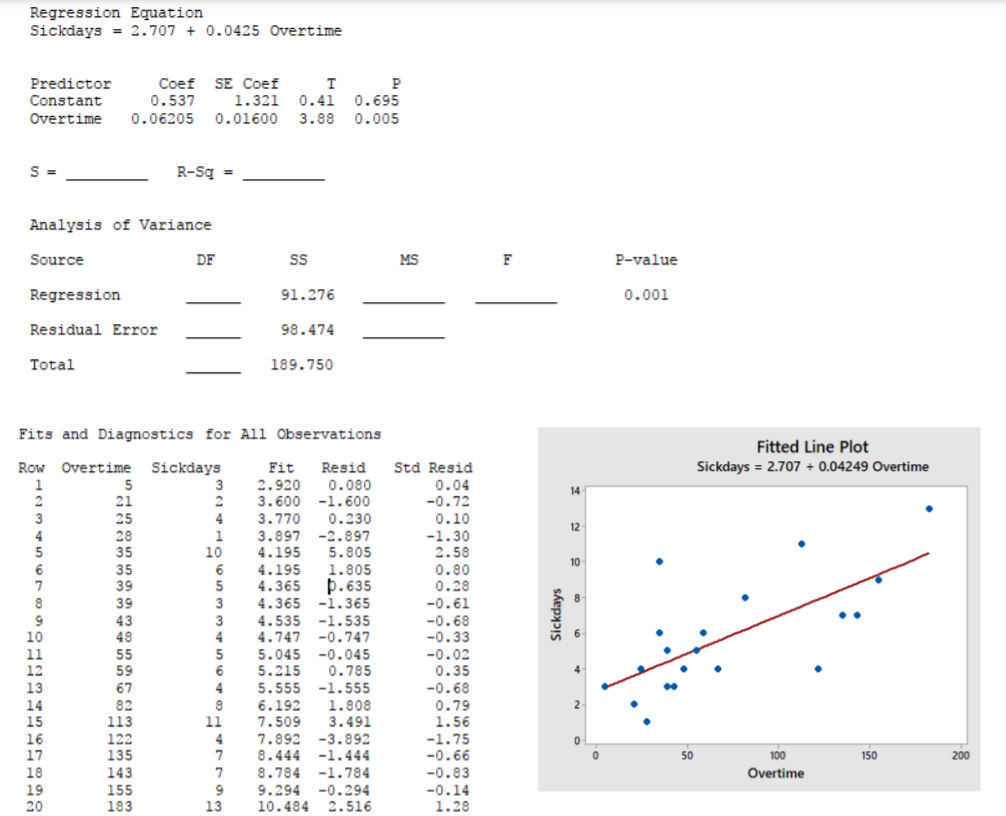
A manager is concerned that overtime (measured in hours) is contributing to more sickness (measured in sick days) among the employees. Data records for 20 employees were sampled with the MINITAB results shown at the end of the questions.
1. Identify the explanatory (Independent) Variable – include units.
2. Identify the response (dependent) variable – include units.
3. Find the least square line where Sick Days is dependent on Overtime. Interpret the slope using the appropriate units.
4. Test the hypothesis that the regression model is significant (\(\alpha = .10\)). Show all steps. Fill in the missing values on the ANOVA table.
5. Find and interpret the \(r^2\), coefficient of determination. (Blank Line)
6. Find the estimate of standard deviation of the residual error. (Blank Line)
7. Identify any residual that is more than two standard deviations from the regression line.

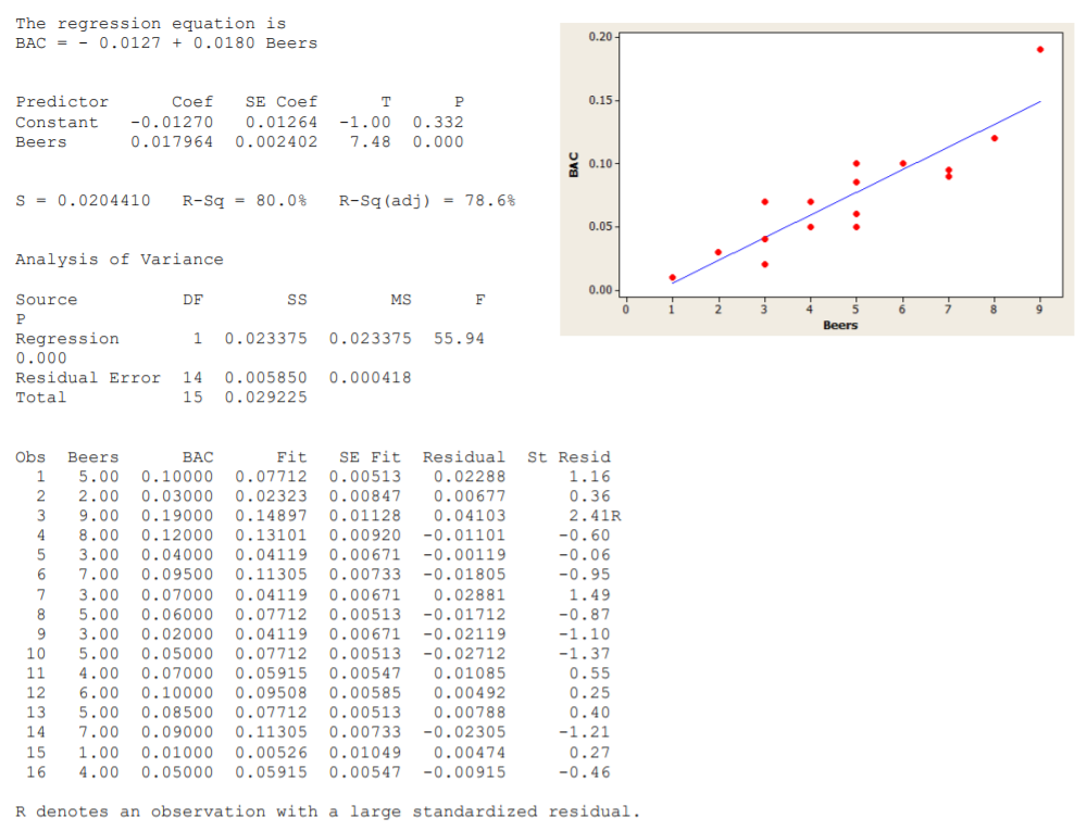
16 student volunteers drank a randomly assigned number of cans of beer. Thirty minutes later a police officer measured their blood alcohol content (BAC) in grams of alcohol per deciliter of blood. Data and computer output are given below the questions.
1. Find the least square line where BAC is dependent on Beers consumed. Interpret the slope.
2. Find and interpret the r‐squared statistic.
3. Test the hypothesis that the beers consumed and BAC are correlated (\(\alpha = .05\))
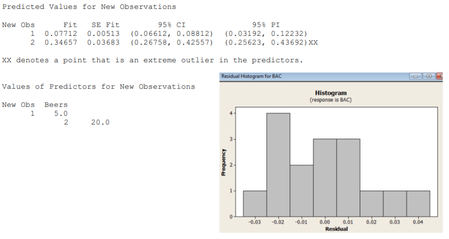
4. Find a 95% Confidence Interval for the mean BAC for a student who consumes 5 beers.
5. Would this model be appropriate for a student who consumed 20 beers? Explain.
6. Joe claims that he can still legally drive after consuming 5 beers: the legal BAC limit is 0.08. Find a 95% Prediction interval for Joe’s BAC. Do you think Joe can legally drive?
7. Residual Analysis
  1. We would expect the residuals to be random: about half would be positive and half would be negative. Check the actual residuals and compare the actual percentages to the expected percentages.
  2. The assumption for regression is that the residuals have a Normal Distribution. This means about 68% of the residuals would have a \(Z\)‐score between ‐1 and 1, 95% of the residuals would have a \(Z\)‐score between ‐2 and 2 and all the residuals would have a Z‐score between ‐3 and 3. The Column labeled “Standardized Residual” is the \(Z\)‐score for each residual. Check to see what percentage of the data has \(Z\)‐scores in each of these three intervals, and compare the actual percentages to the expected percentages (68%, 95%, 100%).

Data for Exercise 4 Regression Analysis: BAC versus Beers

The following regression analysis was used to test Poverty (percentage of population living below the poverty line) as a predictor for Dropout (High School Dropout Percentage.
1. Five items have been blanked out been; find these missing which can be calculated based on other information in the output.
  1. \(r^2\)
  2. \(r\)
  3. Standard Error of the Residuals
  4. \(F\) Test Statistic
  5. Predicted Value for Poverty = 15

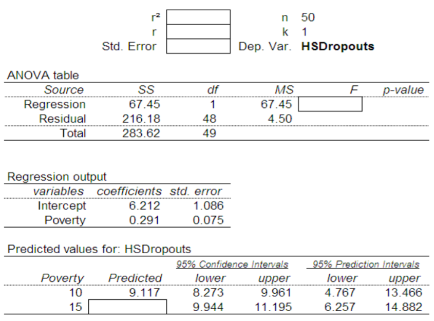
Write out the regression equation.
Conduct the Hypothesis Test that Poverty and HSDropout are correlated with \(\alpha =.01\) (Critical Value for \(F\) is 7.19 (\(\alpha =.01\), DF‐num=1,DF‐den=48)).
What percentage of the variability of High School Dropout Rates can be explained by Poverty?
North Dakota has a Poverty Rate of 11.9 percent and a HS Dropout Rate of 4.6 percent.
1. Calculate the predicted HS Dropout Rate for North Dakota from the regression equation.
2. The Standard Error (from part a‐iii) is the standard deviation with respect to the regression line. Calculate the \(Z\)‐score for the actual North Dakota HS Dropout Rate of 4.6 (Subtract the predicted value and divide by the Standard Error). Do you think that the North Dakota HS Dropout Rate is unusual? Explain.

For the studies in questions 6 to 8:

Identify the explanatory variable.
Identify the response variable
Choose the appropriate model from among these three:
1. Chi‐square test of independence
2. One factor ANOVA
3. Simple Linear Regression

A golf course designer was studying types of grass to be used in a region that was susceptible to droughts. The designer studied 5 types of grass: Bent Grass, Fescue, Rye Grass, Bermuda Grass and Paspalum. Ten samples were taken of each grass and watered to keep the grass in prime condition for a month. For each sample, the daily water usage was calculated in liters per square meter. The designer wanted to know if there was a significant difference in mean water usage due to grass type.
A school psychologist believes students who have more homework will sleep less. 200 students participated in a study. For each of 14 consecutive days, students were asked to count how many minutes they spent doing their homework and how many minutes they slept that night.
Does smoking change the way someone tastes salt? A researcher sampled 200 smokers and 200 non‐smokers. They were then given a bowl of soup and ask to classify the salt level into one of 3 categories: low salt, average salt and high salt. The researcher wanted to know if there was a significant difference in the saltiness classification due to whether the participant was a smoker.