
11.2: Independent Sampling Models
- Page ID
- 20914

We will first consider the case when we want to compare the population means of two populations using independent sampling.
Distribution of the difference of two sample means
Suppose we wanted to test the hypothesis \(H_o: \mu_{1}=\mu_{2}\). We have point estimators for both \(\mu_{1}\) and \(\mu_{2}\), namely \(\overline{X}_1\) and \(\overline{X}_1\), which have approximately Normal Distributions under the Central Limit Theorem, but it would useful to combine them both into a single estimator. Fortunately it is known that if two random variables have a Normal Distribution, then so does the sum and difference. Therefore we can restate the hypothesis as \(H_o: \mu_{1}-\mu_{2}=0\) and use the difference of sample means \(\overline{X}_1 - \overline{X}_1\)as a point estimator for the difference in population means \(\mu_{1}-\mu_{2}\).
We will first consider the case when we want to compare the population means of two populations using independent sampling.
Distribution of the difference of two sample means
Suppose we wanted to test the hypothesis \(H_o: \mu_{1}=\mu_{2}\). We have point estimators for both \(\mu_{1}\) and \(\mu_{2}\), namely \(\overline{X}_1\) and \(\overline{X}_1\), which have approximately Normal Distributions under the Central Limit Theorem, but it would useful to combine them both into a single estimator. Fortunately it is known that if two random variables have a Normal Distribution, then so does the sum and difference. Therefore we can restate the hypothesis as \(H_o: \mu_{1}-\mu_{2}=0\) and use the difference of sample means \(\overline{X}_1 - \overline{X}_2\) as a point estimator for the difference in population means \(\mu_{1}-\mu_{2}\).
\(\mu_{\overline{X}_{1}-\overline{X}_{2}}=\mu_{1-} \mu_{2}\)
\(\sigma_{\overline{X}_{1}-\overline{X}_{2}}=\sqrt{\dfrac{\sigma_{1}^{2}}{n_{1}}+\dfrac{\sigma_{2}^{2}}{n_{2}}}\)
\(Z=\dfrac{\left(\overline{X}_{1}-\overline{X}_{2}\right)-\left(\mu_{1}-\mu_{2}\right)}{\sqrt{\frac{\sigma_{1}^{2}}{n_{1}}+\frac{\sigma_{2}^{2}}{n_{2}}}}\) if \(n_1\) and \(n_2\) are sufficiently large.
Comparing two means, independent sampling: Model when population variances known
When the population variances are known, the test statistic for the Hypothesis \(H_o: \mu_{1}=\mu_{2}\) can be tested with Normal distribution \(Z\) test statistic shown above. Also, if both sample size \(n_1\) and \(n_2\) exceed 30, this model can also be used.
Example: Homes and pools
Are larger homes more likely to have pools? The square footage (size) data for single family homes in California was separated into two populations: Homes with pools and homes without pools. We have data from 130 homes with pools and 95 homes without pools.

Solution
Design
Research Hypotheses:
\(H_o: \mu_{1} \leq \mu_{2}\) (Homes with pools do not have more mean square footage)
\(H_a: \mu_{1} > \mu_{2}\) (Homes with pools do have more mean square footage)
Since both sample sizes are over 30, the model will be a Large sample \(Z\) test comparing two population means with independent sampling.
This model is appropriate since the sample sizes assures the distribution of the sample mean is approximately Normal from the Central Limit Theorem. We opt for a one‐tailed test since we want to support the claim that homes with pools are larger. The test statistic will be \(=\dfrac{\left(\overline{X}_{1}-\overline{X}_{2}\right)-\left(\mu_{1}-\mu_{2}\right)}{\sqrt{\frac{\sigma_{1}^{2}}{n_{1}}+\frac{\sigma_{2}^{2}}{n_{2}}}}\)
Type I error would be to reject the Null Hypothesis and claim home with pools are larger, when they are not larger. It was decided to limit this error by setting the level of significance (\(\alpha\)) to 1%.
The decision rule under the critical value method would be to reject the Null Hypothesis when the value of the test statistic is in the rejection region. In other words, reject \(H_o\) when \(Z > 2.326\). The decision under the \(p\)‐value method is to reject \(H_o\) if the \(p\)‐value is < \(\alpha\).
Data/Results
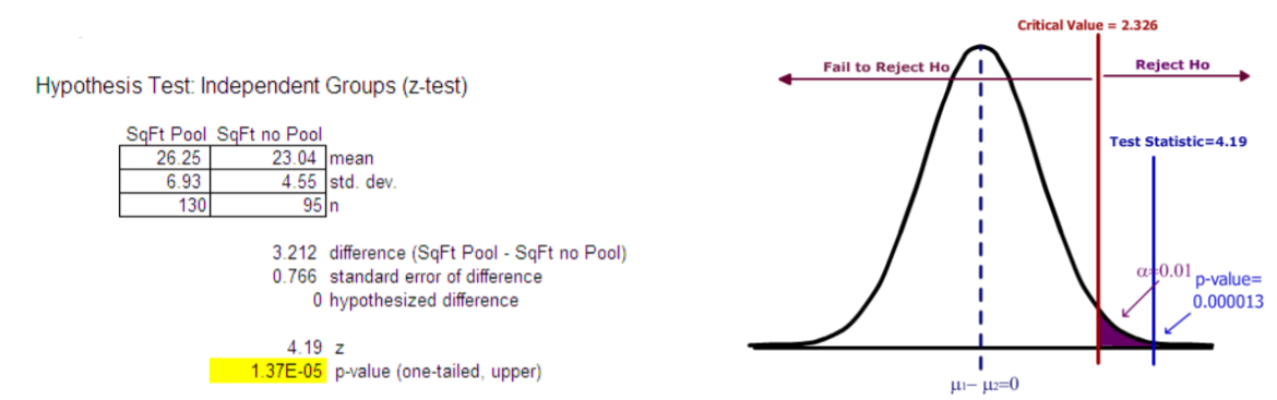
Since the test statistic (\(Z = 4.19\)) is greater than the critical value (2.326), \(H_o\) is rejected. Also the \(p\)‐value (0.000013) is less than \(\alpha\)(0.01), the decision is to Reject \(H_o\).
Conclusion
The researcher makes the strong statement that homes with pools have a significantly higher mean square footage than home without pools.
Model when population variances are unknown, but are assumed to be equal
In the case that the population standard deviations are unknown, it seems logical to simply replace the population standard deviations for each population with the sample standard deviations and use a \(t\)‐distribution as we did for the one population case. However, this is not so simple when the sample size for either group is under 30
We will consider two models. This first model (which we prefer to use since it has more power) assumes the population variances are equal and is called the pooled variance \(t\)‐test. In this model we combine or “pool” the two sample standard deviations into a single estimate called the pooled standard deviation, \(s_p\). If the central limit theorem is working, we then can substitute \(s_p\) for \(s_1\) and \(s_2\) get a \(t\)‐distribution with \(n_{1}+n_{2}-2\) degrees of freedom:
Model Assumptions
- Independent Sampling
- \(\overline{X}_{1}-\overline{X}_{2}\) approximately Normal
- \(\sigma_{1}^{2}=\sigma_{2}^{2}\)
Test Statistic
- \(t=\dfrac{\left(\overline{X}_{1}-\overline{X}_{2}\right)-\left(\mu_{1}-\mu_{2}\right)}{s_{p} \sqrt{\frac{1}{n_{1}}+\frac{1}{n_{2}}}}\)
- \(s_{p}=\sqrt{\dfrac{\left(n_{1}-1\right) s_{1}^{2}-\left(n_{2}-1\right) s_{2}^{2}}{n_{1}+n_{2}-2}}\)
- Degrees of freedom \(=n_{1}+n_{2}-2\)
Example: Fuel economy
A recent EPA study compared the highway fuel economy of domestic and imported passenger cars. A sample of 15 domestic cars revealed a mean of 33.7 MPG (mile per gallon) with a standard deviation of 2.4 mpg. A sample of 12 imported cars revealed a mean of 35.7 mpg with a standard deviation of 3.9. At the .05 significance level can the EPA conclude that the MPG is higher for the imported cars?

Solution
Design
It is best to associate the subscript 2 with the control group; in this case we will let domestic cars be population 2.
Research Hypotheses:
\(H_o: \mu_{1} \leq \mu_{2}\) (Imported compact cars do not have a higher mean MPG)
\(H_a: \mu_{1} > \mu_{2}\) (Imported compact cars have a higher mean MPG)
We will assume the population variances are equal \(\sigma_{1}^{2}=\sigma_{2}^{2}\), so the model will be a Pooled variance \(t\)‐test. This model is appropriate if the distribution of the differences of sample means is approximately Normal from the Central Limit Theorem. A one‐tailed test is selected based on \(H_a\).
Type I error would be to reject the Null Hypothesis and claim that imports have a higher mean MPG, when they do not have higher MPG. The test will be run at a level of significance (\(\alpha\)) of 5%.
The degrees of freedom for this test is 25, so the decision rule under the critical value method would be to reject \(H_o\) when \(t > 1.708\). The decision under the \(p\)‐value method is to reject \(H_o\) if the \(p\)‐value is < \(\alpha\).
Data/Results
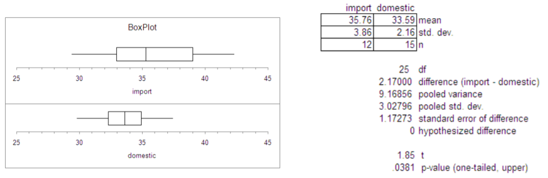
\(s_{p}=\sqrt{\dfrac{(12-1) 3.86^{2}-(12-1) 2.16^{2}}{15+12-2}}=3.03\)
\(t=\dfrac{(35.76-33.59)-0}{3.03 \sqrt{\frac{1}{12}+\frac{1}{15}}}=1.85\)
Since 1.85 > 1.708, the decision would be to Reject \(H_o\). Also the p‐value is calculated to be .0381 which again shows that the result is significant at the 5% level.
Conclusion
Imported compact cars have a significantly higher mean MPG rating when compared to domestic cars
Model when population variances unknown, but assumed to be unequal
In the prior example, we assumed the population variances were equal. However, when looking at the box plot of the data or the sample standard deviations, it appears that the import cars have more variability MPG than domestic cars, which would violate the assumption of equal variances required for the Pooled Variance \(t\)‐test.
Fortunately, there is an alternative model that has been developed for when population variances are unequal, called the Behrens‐Fisher model 81, or the unequal variances \(t\)‐test.
Model Assumptions
- Independent Sampling
- \(\overline{X}_{1}-\overline{X}_{2}\) approximately Normal
- \(\sigma_{1}^{2} \neq \sigma_{2}^{2}\)
Test Statistic
- \(t^{\prime}=\dfrac{\left(\bar{X}_{1}-\bar{X}_{2}\right)-\left(\mu_{1}-\mu_{2}\right)}{\sqrt{\frac{s_{1}^{2}}{n_{1}}+\frac{s_{2}^{2}}{n_{2}}}}\)
- \(d f=\dfrac{\left(\frac{s_{1}^{2}}{n_{1}}+\frac{s_{2}^{2}}{n_{2}}\right)^{2}}{\left[\frac{\left(s_{1}^{2} / n_{1}\right)^{2}}{\left(n_{1}-1\right)}+\frac{\left(s_{2}^{2} / n_{2}\right)^{2}}{\left(n_{2}-1\right)}\right]}\)
The degrees of freedom will be less than or equal to \(n_{1}+n_{2}-2\), so this test will usually have less power than the pooled variance \(t\)‐test.
Example: Fuel economy
We will repeat the prior example to see if we can support the claim that imported compact cars have higher mean MPG when compared to domestic compact cars. This time we will assume that the population variances are not equal.
Solution
Design
Again we will let domestic cars be population 2.
Research Hypotheses:
\(H_o: \mu_{1} \leq \mu_{2}\) (Imported compact cars do not have a higher mean MPG)
\(H_a: \mu_{1} > \mu_{2}\) (Imported compact cars have a higher mean MPG)
We will assume the population variances are unequal \(\sigma_{1}^{2} \neq \sigma_{2}^{2}\), so the model will be an unequal variance \(t\)‐test. This model is appropriate if the distribution of the differences of sample means is approximately Normal from the Central Limit Theorem. A one‐tailed test is selected based on \(H_a\).
Type I error would be to reject the Null Hypothesis and claim imports have a higher mean MPG, when they do not have higher MPG. The test will be run at a level of significance (\(\alpha\)) of 5%. The degrees of freedom for this test is 16 (see calculation below), so the decision rule under the critical value method would be to reject \(H_o\) when \(t > 1.746\). The decision under the \(p\)‐value method is to reject \(H_o\) if the \(p\)‐value is < \(\alpha\)
Data/Results
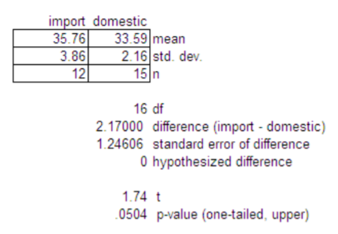
\(d f=\dfrac{\left(\frac{2.16^{2}}{15}+\frac{3.86^{2}}{12}\right)^{2}}{\left[\frac{\left(2.16^{2} / 15\right)^{2}}{(15-1)}+\frac{\left(3.86^{2} / 12\right)^{2}}{(12-1)}\right]}=16\)
\(t=\dfrac{(35.76-33.59)-0}{\sqrt{\frac{2.16^{2}}{15}+\frac{3.86^{2}}{12}}}=1.74\)
Since 1.74 <1.746, the decision would be to Fail to Reject \(H_o\). Also the \(p\)‐value is calculated to be .0504 which again shows that the result is not significant (barely) at the 5% level.
Conclusion
Insufficient evidence to claim imported compact cars have a significantly higher mean MPG rating when compared to domestic cars.
You can see the lower power of this test when compared to the pooled variance \(t\)‐test example where Ho was rejected. We always prefer to run the test with higher power when appropriate.