10.4: Collect and Analyze Experimental Data

Last updated
Save as PDF

Page ID: 20907

\( \newcommand{\vecs}[1]{\overset { \scriptstyle \rightharpoonup} {\mathbf{#1}} } \) \( \newcommand{\vecd}[1]{\overset{-\!-\!\rightharpoonup}{\vphantom{a}\smash {#1}}} \)\(\newcommand{\id}{\mathrm{id}}\) \( \newcommand{\Span}{\mathrm{span}}\) \( \newcommand{\kernel}{\mathrm{null}\,}\) \( \newcommand{\range}{\mathrm{range}\,}\) \( \newcommand{\RealPart}{\mathrm{Re}}\) \( \newcommand{\ImaginaryPart}{\mathrm{Im}}\) \( \newcommand{\Argument}{\mathrm{Arg}}\) \( \newcommand{\norm}[1]{\| #1 \|}\) \( \newcommand{\inner}[2]{\langle #1, #2 \rangle}\) \( \newcommand{\Span}{\mathrm{span}}\) \(\newcommand{\id}{\mathrm{id}}\) \( \newcommand{\Span}{\mathrm{span}}\) \( \newcommand{\kernel}{\mathrm{null}\,}\) \( \newcommand{\range}{\mathrm{range}\,}\) \( \newcommand{\RealPart}{\mathrm{Re}}\) \( \newcommand{\ImaginaryPart}{\mathrm{Im}}\) \( \newcommand{\Argument}{\mathrm{Arg}}\) \( \newcommand{\norm}[1]{\| #1 \|}\) \( \newcommand{\inner}[2]{\langle #1, #2 \rangle}\) \( \newcommand{\Span}{\mathrm{span}}\)\(\newcommand{\AA}{\unicode[.8,0]{x212B}}\)

After designing the experiment, we would then collect and verify the data. For the purposes of statistical analysis, we will assume that all sampling is either random or uses an alternative technique that adequately simulates a random sample.

Data Verification

After collecting the data but before running the test, we need to verify the data. First, get a picture of the data by making a graph (histogram, dot plot, box plot, etc). Check for skewness, shape and any potential outliers in the data.

Working with Outliers

An outlier is a data point that is far removed from the other entries in the data set. Outliers could be caused by:

Mistakes made in recording data
Data that don’t belong in population
True rare events

The first two cases are simple to deal with since we can correct errors or remove data that does not belong in the population. The third case is more problematic as extreme outliers will increase the standard deviation dramatically and heavily skew the data.

In The Black Swan, Nicholas Taleb argues that some populations with extreme outliers should not be analyzed with traditional confidence intervals and hypothesis testing.⁷² He defines a Black Swan to be an unpredictable extreme outlier that causes dramatic effects on the population. A recent example of a Black Swan was the catastrophic drop in the value of unregulated Credit Default Swap (CDS) real estate insurance investments causing the near collapse of the international banking system in 2008. The traditional statistical analysis that measured the risk of the CDS investments did not take into account the consequence of a rapid increase in the number of foreclosures of homes. In this case, statistics that measure investment performance and risk were useless and created a false sense of security for large banks and insurance companies.

Example: Realtor home sales

Here are the quarterly home sales for 10 realtors

2 2 3 4 5 5 6 6 7 50

	With outlier	Without outlier
Mean	9.00	4.44
Median	5.00	5.00
Standard Deviation	14.51	1.81
Interquartile Range	3.00	3.50

In this example, the number 50 is an outlier. When calculating summary statistics, we can see that the mean and standard deviation are dramatically affected by the outlier, while the median and the interquartile range (which are based on the ranking of the data) are hardly changed. One solution when dealing with a population with extreme outliers is to use inferential statistics using the ranks of the data, also called non‐parametric statistics.

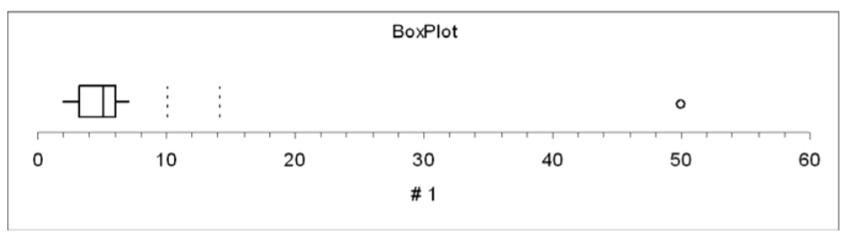
Using Box Plot to find outliers

The “box” is the region between the 1st and 3rd quartiles.
Possible outliers are more than 1.5 IQR’s from the box (inner fence)
Probable outliers are more than 3 IQR’s from the box (outer fence)
In the box plot below, which illustrates the realtor example, the dotted lines represent the “fences” that are 1.5 and 3 IQR’s from the box. See how the data point 50 is well outside the outer fence and therefore an almost certain outlier.

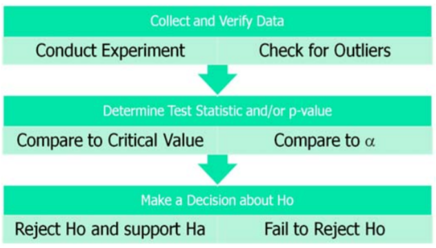
The Logic of Hypothesis Testing

After the data is verified, we want to conduct the hypothesis test and come up with a decision: whether or not to reject the Null Hypothesis. The decision process is similar to a “proof by contradiction” used in mathematics:

We assume Ho is true before observing data and design \(H_{a}\) to be the complement of \(H_{o}\).
Observe the data (evidence). How unusual are these data under \(H_{o}\)?
If the data are too unusual, we have “proven” \(H_{o}\) is false: reject \(H_{o}\) and support \(H_{a}\) (strong statement).
If the data are not too unusual, we fail to reject \(H_{o}\). This “proves” nothing and we say data are inconclusive. (weak statement) .
We can never “prove” \(H_{o}\), only “disprove” it.
“Prove” in statistics means support with (\(1-\alpha\))100% certainty. (example: if \(\alpha =.05\), then we are at least 95% confident in our decision to reject \(H_{o}\).

Decision Rule – Two methods, Same Decision

Earlier we introduced the idea of a test statistic which is a value calculated from the data under the appropriate Statistical Model from the data that can be compared to the critical value of the Hypothesis test. If the test statistic falls in the rejection region of the statistical model, we reject the Null Hypothesis.

Recall that the critical value was determined by design on the basis of the chosen level of significance \(\alpha\). The more preferred method of making decisions is to calculate the probability of getting a result as extreme as the value of the test statistic. This probability is called the \(p\)‐value, and can be compared directly to the significance level.

Definition: \(p\)-value

\(p\)‐value: the probability, assuming that the null hypothesis is true, of getting a value of the test statistic at least as extreme as the computed value for the test.

If the \(p\)‐value is smaller than the significance level \(\alpha\), \(H_o\) is rejected.
If the \(p\)‐value is larger than the significance level \(\alpha\), \(H_o\) is not rejected.

Comparing \(p\)‐value to \(\alpha\)

Both the \(p\)‐value and \(\alpha\) are probabilities of getting results as extreme as the data assuming \(H_o\) is true.

The \(p\)‐value is determined by the data and is related to the actual probability of making Type I error (rejecting a true Null Hypothesis). The smaller the \(p\)‐value, the smaller the chance of making Type I error and therefore, the more likely we are to reject the Null Hypothesis.

The significance level \(\alpha\) is determined by the design and is the maximum probability we are willing to accept of rejecting a true \(H_o\).

Two Decision Rules lead to the same decision.

If the test statistic lies in the rejection region, reject \(H_o\). (critical value method)
If the \(p\)‐value < \(\alpha\), reject \(H_o\). (\(p\)‐value method)

This \(p\)‐value method of comparison is preferred to the critical value method because the rule is the same for all statistical models: Reject \(H_o\) if \(p\)‐value < \(\alpha\).

Let’s see why these two rules are equivalent by analyzing a test of mean vs. hypothesized value.

Decision is Reject \(H_o\)

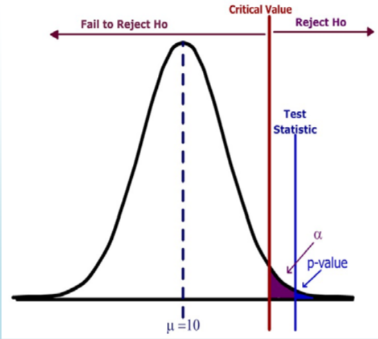
\( H_o: \mu=10 \qquad H_a: \mu > 10\)
Design: Critical value is determined by significance level \(\alpha\).
Data Analysis: p‐value is determined by test statistic
Test statistic falls in rejection region.
\(p\)‐value (blue) < \(\alpha\) (purple)
Reject \(H_o\).
Strong statement: Data supports the Alternative Hypothesis.

In this example, the test statistic lies in the rejection region (the area to the right of the critical value). The \(p\)‐value (the area to the right of the test statistic) is less than the significance level (the area to the right of the critical value). The decision is to Reject \(H_o\).

Decision is Fail to Reject \(H_o\)

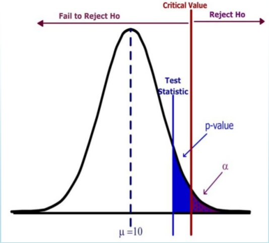
\( H_o: \mu=10 \qquad H_a: \mu > 10\)
Design: critical value is determined by significance level \(\alpha\).
Data Analysis: \(p\)‐value is determined by test statistic
Test statistic does not fall in the rejection region.
\(p\)‐value (blue) > \(\alpha\)(purple)
Fail to Reject \(H_o\).
Weak statement: Data is inconclusive and does not support the Alternative Hypothesis.

In this example, the Test Statistic does not lie in the Rejection Region. The \(p\)‐value (the area to the right of the test statistic) is greater than the significance level (the area to the right of the critical value). The decision is Fail to Reject \(H_o\).