7.4: Normal Distribution
- Page ID
- 20898

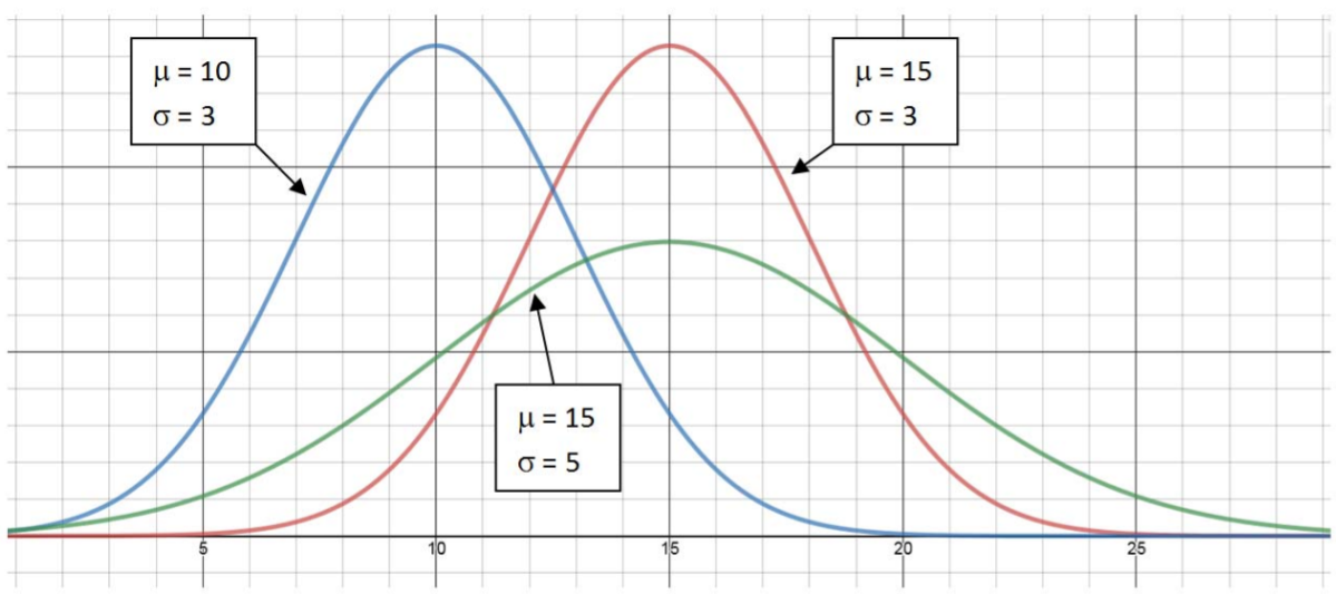
The most important probability distribution in Statistics is the Normal Distribution, the iconic bell‐ shaped curve. The Normal Distribution is symmetric and defined by two parameters: the expected value (mean) \(\mu\) which describes the center of the distribution and the standard deviation \(\sigma\), which describes the spread.
The extremely complicated probability distribution function for the Normal Distribution is:
\[f(x)=\dfrac{1}{\sigma \sqrt{2 \pi}} e^{-\frac{1}{2}\left(\frac{x-\mu}{\sigma}\right)^{2}},-\infty<X<\infty \nonumber \]
Examples of the Normal Distribution are shown here.
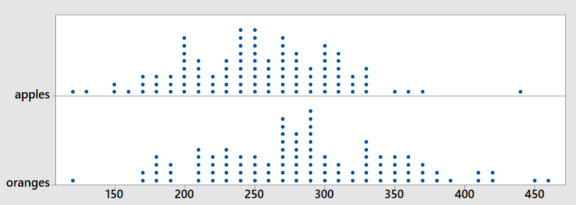
There are many examples of data that are both symmetric and clustered towards the mean. For example, we created dot plots of the weights of apples and oranges in Chapter 2. You can see both graphs are clustered towards the center and are symmetric. A Normal Distribution would be an appropriate model for weight of apples and oranges
Standard Normal Distribution
A special case of the Normal Distribution is when \(\mu=0\) and \(\sigma=1\).
This random variable is known as the Standard Normal Distribution and is always represented by the letter \(Z\).
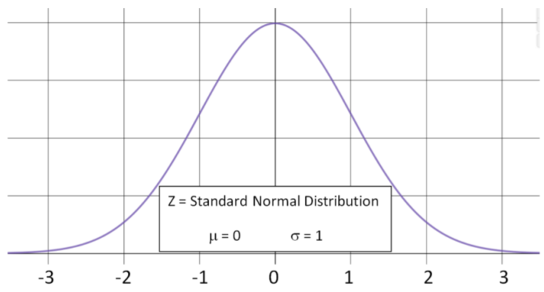
For calculating probabilities and percentiles of the Normal Distribution, tables, graphing calculators or computers are needed. For illustration purposes, we will fill in some of the these probabilities for the Standard Normal Distribution by showing areas under the curve:
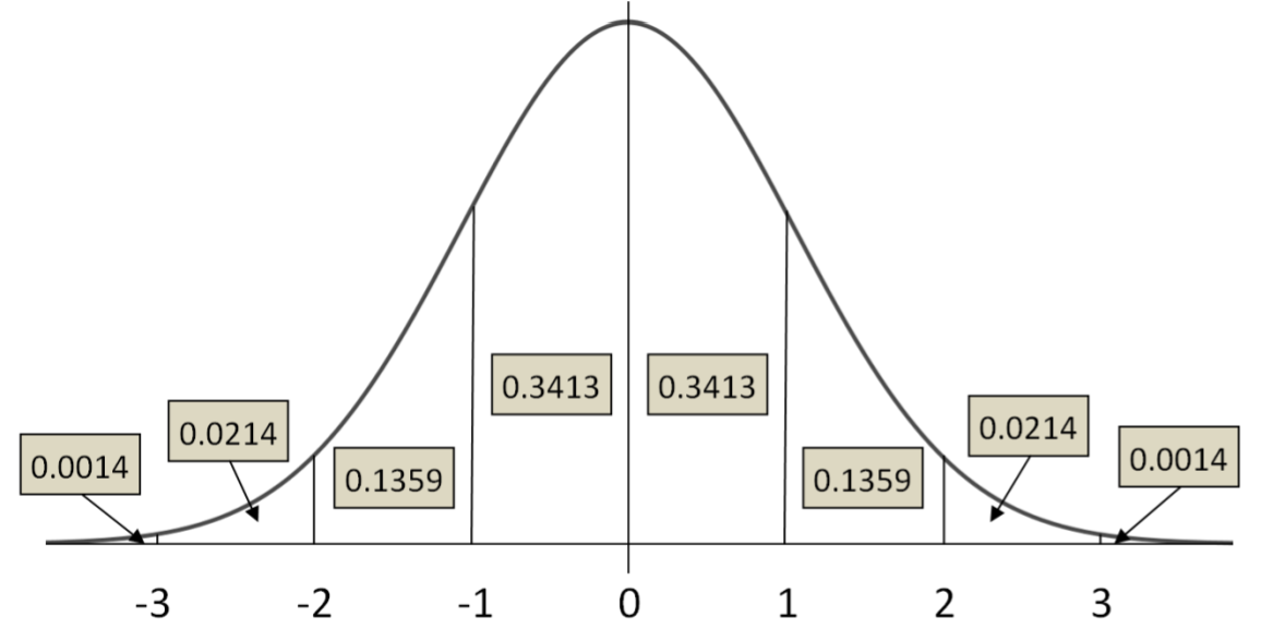
\(P(-1<Z<1)=0.3413+0.3413=0.6826\)
\(P(-2<Z<2)=0.3413+0.3413+0.1359+0.1359=0.9544\)
\(P(-3<Z<3)=0.3413+0.3413+0.1359+0.1359+0.0214+0.0214=0.9972\)
This means that for the standard Normal Distribution that 68% of the probability is between 1 and ‐1, 95% of the probability is between ‐2 and 2 and 99.7% of the probability is between ‐3 and 3.
These percentages may seem familiar from the Empirical Rule in Chapter 3.
68% of the data is within 1 standard deviation of the mean.
95% of the data is within 2 standard deviations of the mean.
99.7% of the data is within 3 standard deviations of the mean.
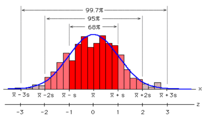
The Empirical Rule comes directly from the Standard Normal Distribution, \(Z\). In fact, any Normal Random Variable, \(X\) with Expected value \(\mu\) and Standard Deviation \(\sigma\) can be converted to a Standard Normal Distribution by using the formula: \(Z=\dfrac{X-\mu}{\sigma}\)
Example: Water usage
The daily water usage per person in a town is normally distributed with a mean (expected value) of 20 gallons and a standard deviation of 5 gallons.
- Determine the proportion of people who use between 15 and 25 gallons of water.
- Determine the proportion of people who use between 10 and 30 gallons of water
- Between what two values would you expect to find about 95% of the water users?
Solution
- \(\begin{aligned}
P(15<X<25) &=P\left(\dfrac{15-20}{5}<Z<\dfrac{25-20}{5}\right) \\
&=P(-1<Z<1)\\&=0.6826
\end{aligned}\) - \(\begin{aligned}
P(10<X<30) &=P\left(\dfrac{10-20}{5}<Z<\dfrac{30-20}{5}\right) \\
&=P(-2<Z<2)\\&=0.9544
\end{aligned}\) - Since \(P(-2<Z<2)=0.9544\), we can say about 95% of the water users are within two standard deviation of the mean, or that they use between 10 and 30 gallons per day.
Normal Probability Distribution (parameters: \(\mu, \sigma\))
\(\mu\) = Expected Value of X, population mean
\(\sigma\) = population standard deviation
\(f(x)=\dfrac{1}{\sigma \sqrt{2 \pi}} e^{-\frac{1}{2}\left(\frac{x-\mu}{\sigma}\right)^{2}},-\infty<X<\infty\)
| Calculating Probabilities | Calculating Percentiles |
|---|---|
|
\(Z=\dfrac{X-\mu}{\sigma}\)
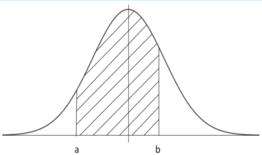
\(P(a<X<b)=P\left(\dfrac{a-\mu}{\sigma}<Z<\dfrac{b-\mu}{\sigma}\right)\) |
\(X=\mu+Z \sigma\)
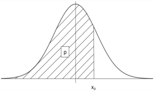
\(P\left(Z<z_{p}\right)=P\left(X<\mu+z_{p} \sigma\right)=p\) |
In general, probability and percentile questions using the Normal Distribution will require a tables or technology that can calculate Normal Distribution probabilities or percentiles for non‐integer \(Z\) values
Example: Water usage
The daily water usage per person in a town is normally distributed with a mean of 20 gallons and a standard deviation of 5 gallons.
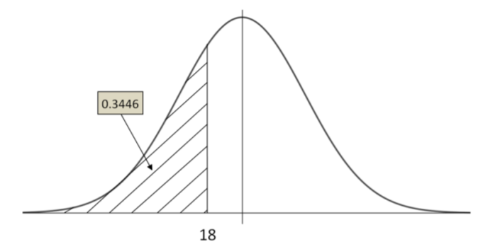
- What is the probability that a person from the town selected at random will use fewer than 18 gallons per person per day?
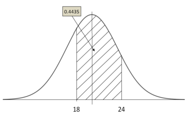
- What proportion of the people use between 18 and 24 gallons per person per day?
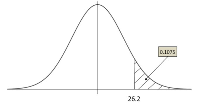
- What percentage of the population uses more than 26.2 gallons per person per day?
- A special tax is going to be charged on the top 5% of water users. Find the value of daily water usage that generates the special tax.
Solution
- \(\begin{aligned}
P(X<18) &=P\left(Z<\dfrac{18-20}{5}\right) \\
&=P(Z<-0.40)\\&=0.3446
\end{aligned}\)
- \(\begin{aligned}
P(18<X<24) &=P\left(\dfrac{18-20}{5}<Z<\dfrac{24-20}{5}\right) \\
&=P(-0.40<Z<0.80)\\&=0.4435
\end{aligned} \)
- \(\begin{aligned}
P(X>26.2) &=P\left(Z>\dfrac{26.2-20}{5}\right) \\
&=P(Z>1.24)\\&=10.75 \%
\end{aligned} \)
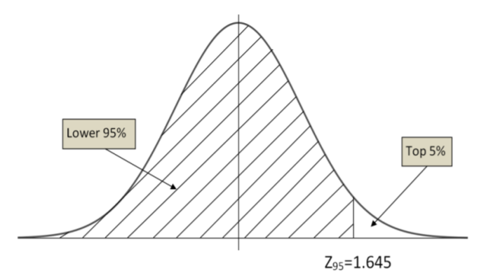
- This problem is really finding the \(95^{th}\) percentile.
The \(Z\) value associated with \(95^{th}\) percentile =1.645
\(X_{95}=20 + 5(1.645) = 28.2\) gallons per day
Example: Grading on the curve
Professor Kurv has determined that the final averages in his statistics course is normally distributed with a mean of 77.1 and a standard deviation of 11.2. He decides to assign his grades for his current course such that the top 15% of the students receive an A.
What is the lowest average a student can receive to earn an A?
Solution
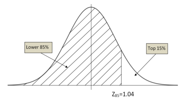
The top 15% would be the finding the \(85^{th}\) percentile. The corresponding \(Z\) value is 1.04.
The minimum grade for an A: \(X=77.1+(1.04)(11.2)\), or \(X=88.75\) points.
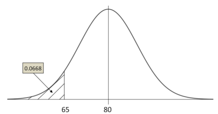
Example: Server tip
The amount of tip the servers in an exclusive restaurant receive per shift is normally distributed with a mean of $80 and a standard deviation of $10. Shelli feels she has provided poor service if her total tip for the shift is less than $65. (This doesn't mean she gave poor service, but rather that she just feels like she did).
What percentage of the time will she feel like she provided poor service?
Solution
Let \(y\) be the amount of tip.
The \(Z\) value associated with \(X=65\) is \(Z= (65‐80)/10= ‐1.5\).
Thus \(P(X<65)=P(Z<-1.5)=.0668\)