7.2: Exponential Distribution

The exponential distribution is often used to model the waiting time until an event occurs. For example, the waiting time until you receive a text message or the waiting time until an accident at a manufacturing plant will follow an exponential distribution.

This model has one parameter, the expected waiting time, \(\mu\).  

An important assumption for the Exponential is that the expected future waiting time is independent of the past waiting time. For example, if you expect to wait 5 minutes for a text message and you wait 3 minutes, the expected waiting time at that point is still 5 minutes.

This can be written as a probability statement: \(P(X>a)=P(X>a+b \mid X>b)\)

The Exponential Distribution is useful to model the waiting time until something “breaks”, but would not be the appropriate model for something that “wears out.”

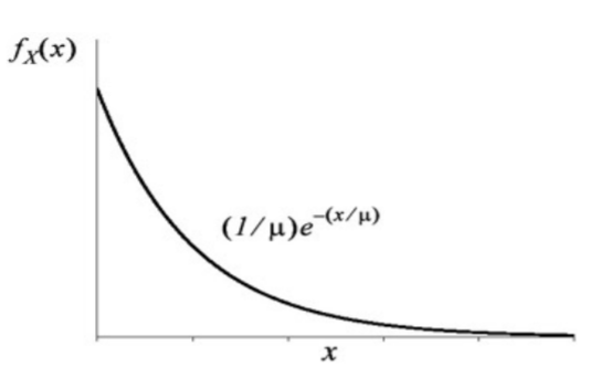
Exponential Probability Distribution (parameter=\(\mu\))

\(\mu\) = expected waiting time until event occurs.

\(X\) = waiting time until event occurs

Assumption: Waiting time in the future is independent of waiting time in the past:

\(P(X>a)=P(X>a+b \mid X>b)\)

\(\sigma^{2}=\mu^{2}\)

\(\sigma=\mu\)

Example: Cracked screen on smart phone.

The time until a screen is cracked on a smart phone has an Exponential distribution with \(\mu=500\) hours of use.

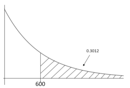
1. Find the probability that the screen will not crack for at least 600 hours.
2. What is the median time until the smart phone's screen is cracked?

Solution

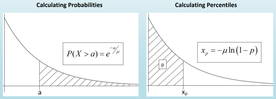
1. Here we use the formula for a probability problem, \(P(X>a)=e^{-a / \mu}\)

\[P(x>600)=e^{-600 / 500}=e^{-1.2}=.3012 \nonumber \]

Assuming that the screen has already lasted 500 hours without cracking, find the chance that the display will last an additional 600 hours.

Because of the memoryless feature of the Exponential distribution, the answer will be the same as if the smart phone was never used.

\[P(x>1100 \mid x>500)=P(x>600)=.3012 \nonumber \]

2. Because the Exponential distribution is always positively skewed, the median will be lower than the mean of 500 hours. The median is the \(50^{th}\) percentile, so this is a percentile problem. We can derive the formula for the \(p^{th}\) percentile (\(x_p\)) using algebra:

\[\begin{aligned}
P\left(X>x_{p}\right)=e^{-x_{p} / \mu}&=1-p \\
-x_{p} / \mu&=\ln (1-p) \\
x_{p}&=-\mu \ln (1-p)
\end{aligned} \nonumber \]

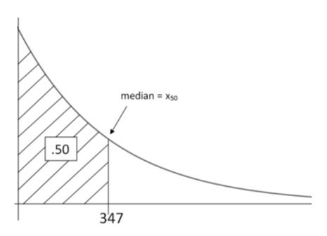
median \(=x_{50}=-500 \ln (1-0.5)=347\) hours

This means that half of smart phones will have cracked screens after 347 hours of usage.

Relationship between Exponential Distribution and Poisson Distribution

There is a relationship between the Poisson Distribution, (covered in Chapter 6 on discrete distributions) and the Exponential Distribution. Recall that the Poisson distributions models  the number of occurrences in a fixed time period if the rate that events occur follows a constant rate. A random variable that follows a Poisson Distribution is called a Poisson Process.

If occurrences follow a Poisson Process with mean = \(\mu\), then the waiting time for the next occurrence has Exponential distribution with mean = \(1 / \mu\).

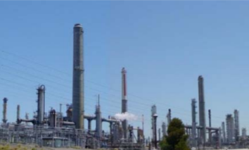
Example: Accidents at an oil refinery⁶⁸

Accidents occur at an oil refinery at a constant rate of 3 per month. This is an example of a Poisson Process.

The random variable \(Y\) = the number of accidents in the next month would follow a Poisson Distribution with \(\mu=3\) occurrences per month

The Random Variable \(X\) = the waiting time until the next refinery accident would follow an Exponential distribution with \(\mu=1 / 3\) months.

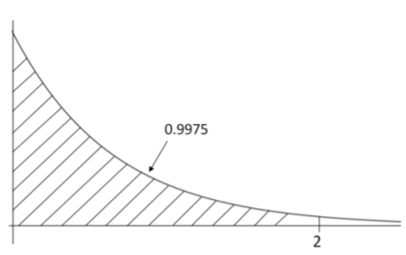
1. Find the probability of waiting less than 2 months for the next oil refinery accident.
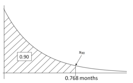
2. Find the \(90^{th}\) percentile of waiting times for a refinery accident

Solution

1. \(P(X<2)=1-e^{-2 /(1 / 3)}=1-e^{-6}=0.9975\)

2. \(x_{95}=-\dfrac{1}{3} \ln (1-.90)=0.768\) months