7.1: What is a Continuous Random Variable?

Last updated
Save as PDF

Page ID: 20895

\( \newcommand{\vecs}[1]{\overset { \scriptstyle \rightharpoonup} {\mathbf{#1}} } \) \( \newcommand{\vecd}[1]{\overset{-\!-\!\rightharpoonup}{\vphantom{a}\smash {#1}}} \)\(\newcommand{\id}{\mathrm{id}}\) \( \newcommand{\Span}{\mathrm{span}}\) \( \newcommand{\kernel}{\mathrm{null}\,}\) \( \newcommand{\range}{\mathrm{range}\,}\) \( \newcommand{\RealPart}{\mathrm{Re}}\) \( \newcommand{\ImaginaryPart}{\mathrm{Im}}\) \( \newcommand{\Argument}{\mathrm{Arg}}\) \( \newcommand{\norm}[1]{\| #1 \|}\) \( \newcommand{\inner}[2]{\langle #1, #2 \rangle}\) \( \newcommand{\Span}{\mathrm{span}}\) \(\newcommand{\id}{\mathrm{id}}\) \( \newcommand{\Span}{\mathrm{span}}\) \( \newcommand{\kernel}{\mathrm{null}\,}\) \( \newcommand{\range}{\mathrm{range}\,}\) \( \newcommand{\RealPart}{\mathrm{Re}}\) \( \newcommand{\ImaginaryPart}{\mathrm{Im}}\) \( \newcommand{\Argument}{\mathrm{Arg}}\) \( \newcommand{\norm}[1]{\| #1 \|}\) \( \newcommand{\inner}[2]{\langle #1, #2 \rangle}\) \( \newcommand{\Span}{\mathrm{span}}\)\(\newcommand{\AA}{\unicode[.8,0]{x212B}}\)

A continuous random variable is a random variable that has only continuous values. Continuous values are uncountable and are related to real numbers.

Examples of continuous random variables

The time it takes to complete an exam for a 60 minute test Possible values = all real numbers on the interval [0,60]
Age of a fossil Possible values = all real numbers on the interval [minimum age, maximum age]
Miles per gallon for a Toyota Prius Possible Values = all real numbers on the interval [minimum MPG, maximum MPG]

The main difference between continuous and discrete random variables is that continuous probability is measured over intervals, while discrete probability is calculated on exact points.

For example, it would make no sense to find the probability it took exactly 32 minutes to finish an exam. It might take you 32.012342472… minutes. Probability of points no longer makes sense when we move from discrete to continuous random variables.

Instead, you could find the probability of taking at least 32 minutes for the exam, or the probability of taking between 31 and 33 minutes to complete the exam. Instead of assigning probability to points, we instead define a probability density function (pdf) that will help us find probabilities. This function must always have a non‐negative range (output). Probability can then be determined by finding the area under the function. To be a valid probability density function, the total area under the curve must equal 1.

If the drawing represents a valid probability density function for a random variable \(X\), then

\[P(a<X<b)=\text { shaded area } \nonumber \]

This table shows the similarities and differences between Discrete and Continuous Distributions

Discrete Distributions	Continuous Distributions
Countable Discrete Points Points have probability \(p(x)\) is probability distribution function \(p(x) \geq 0\) \(\Sigma p(x)=1\)	Uncountable Continuous Intervals Points have no probability \(f(x)\) is probability density function \(f(x) \geq 0\) Total Area under curve =1

Discrete Distributions

Continuous Distributions

Countable

Discrete Points

Points have probability

\(p(x)\) is probability distribution function

\(p(x) \geq 0\)

\(\Sigma p(x)=1\)

Uncountable

Continuous Intervals

Points have no probability

\(f(x)\) is probability density function

\(f(x) \geq 0\)

Total Area under curve =1

Example: Driving to school

The time to drive to school for a community college student is an example of a continuous random variable. The probability density function and areas of regions created by the points 15 and 25 minutes are shown in the graph.

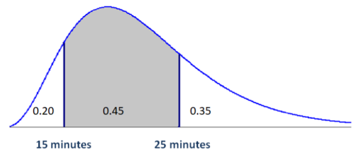
Find the probability that a student takes less than 15 minutes to drive to school.
Find the probability that a student takes no more than 15 minutes to drive to school. This answer is the same as the prior question, because points have no probability with continuous random variables.
Find the probability that a student takes more than 15 minutes to drive to school.
Find the probability that a student takes between 15 and 25 minutes to drive to school.

Solution

\(P(X<15)=0.20\)
\(P(X \leq 15)=0.20\)
\(P(X>15)=0.45+0.35=0.80\)
\(P(15 \leq X \leq 25)=0.45\)

We can also use a continuous distribution model to determine percentiles.

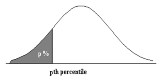
The \(p^{th}\) percentile is the value \(x_p\) such that \(P\left(X<x_{p}\right)=p\)

Find the \(20^{th}\) and \(65^{th}\) percentiles of times driving to school.

From the drawing \(X_{20} = 15\) minutes and \(X_{65} = 25\) minutes

Expected Value and Variance of Continuous Random Variables

The mean and variance can be calculated for most continuous random variables. The actual calculations require calculus and are beyond the scope of this course. We will use the same symbols to define the expected value and variance that were used for discrete random variables.

Expected Value (\(\mu\)) and Variance (\(\sigma^{2}\)) of Continuous Random Variable \(X\)

Expected Value (Population Mean): \(\mu=E(x)\)

Population Variance: \(\sigma^{2}=\operatorname{Var}(x)=E\left[(x-\mu)^{2}\right]\)

Population Standard Deviation: \(\sigma=\sqrt{\operatorname{Var}(x)}\)

These next sections explore three special continuous random variables that have practical applications.