6.8: Poisson Distribution

Last updated
Save as PDF

Page ID: 20894

\( \newcommand{\vecs}[1]{\overset { \scriptstyle \rightharpoonup} {\mathbf{#1}} } \) \( \newcommand{\vecd}[1]{\overset{-\!-\!\rightharpoonup}{\vphantom{a}\smash {#1}}} \)\(\newcommand{\id}{\mathrm{id}}\) \( \newcommand{\Span}{\mathrm{span}}\) \( \newcommand{\kernel}{\mathrm{null}\,}\) \( \newcommand{\range}{\mathrm{range}\,}\) \( \newcommand{\RealPart}{\mathrm{Re}}\) \( \newcommand{\ImaginaryPart}{\mathrm{Im}}\) \( \newcommand{\Argument}{\mathrm{Arg}}\) \( \newcommand{\norm}[1]{\| #1 \|}\) \( \newcommand{\inner}[2]{\langle #1, #2 \rangle}\) \( \newcommand{\Span}{\mathrm{span}}\) \(\newcommand{\id}{\mathrm{id}}\) \( \newcommand{\Span}{\mathrm{span}}\) \( \newcommand{\kernel}{\mathrm{null}\,}\) \( \newcommand{\range}{\mathrm{range}\,}\) \( \newcommand{\RealPart}{\mathrm{Re}}\) \( \newcommand{\ImaginaryPart}{\mathrm{Im}}\) \( \newcommand{\Argument}{\mathrm{Arg}}\) \( \newcommand{\norm}[1]{\| #1 \|}\) \( \newcommand{\inner}[2]{\langle #1, #2 \rangle}\) \( \newcommand{\Span}{\mathrm{span}}\)\(\newcommand{\AA}{\unicode[.8,0]{x212B}}\)

Random variables that can be thought of as “How many occurrences per time period”, or “How many occurrences per region” have many practical applications. For example:

The number of strong earthquakes per year in California.

The number of customers per hour at a restaurant.

The number of accidents per week at a manufacturing plant.

The number of errors per page in a manuscript.

If the rate is constant, these random variables will follow a Poisson distribution.

The Poisson Distribution is actually derived from a Binomial Distribution in which the sample size \(n\) gets very large and the probability of success \(p\) is very small. A good example of this is the Powerball Lottery.

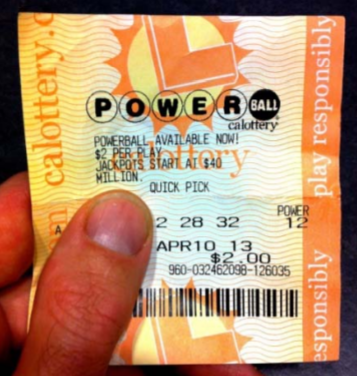
Example: Powerball Lottery

The odds of winning the Powerball Lottery jackpot with a single ticket are 292,000,000 to 1. Suppose the jackpot gets large and 292,000,000 tickets are sold.

Solution

Let \(X\) = Number of jackpot winning tickets sold.

Under the Binomial distribution, \(n=292,000,000\) and \(p = 1/292,000,000\). Note that \(p\) is very close to zero, so \(1‐p\) is very close to 1.

\(\mu=n p=1\)

\(\sigma^{2}=n p(1-p) \approx n p=\mu=1\)

The number of winners can be modeled by the Poisson Distribution, in which the single parameter \(\(\mu\) is the expected number of winners; in this case \(\mu=1\). There could theoretically be millions of winners, so the possible values of the Poisson is designed so there is no theoretical limit for the value of \(X\) (although there are practical limits in real life problems).

The important features of the Poisson Distribution are shown here:

Poisson Probability Distribution (parameter= \(\mu\))

\(\mu\) = expected occurrences per given time period or region. This rate must be constant.

\(X\) = number of occurrence per given time period or region Possible values of \(X\) {0, 1, 2, …} (no upper limit)

\(\sigma^{2}=\mu\)

\(\sigma=\sqrt{\mu}\)

\(P(x)=\dfrac{e^{-\mu} \mu^{x}}{x !}\)

Example: Continuation of Powerball Lottery

Find the probability of no jackpot winners.

\(P(0)=\dfrac{e^{-1} 2^{0}}{0 !}=0.368\)

Find the probability of at least one jackpot winner. The answer calculated directly is an infinite sum, so instead use the Rule of Complement

\(P(X \geq 1)=P(1)+P(2)+\cdots\)

\(P(X \geq 1)=1-P(0)=1-\dfrac{e^{-1} 2^{0}}{0 !}=0.632\)

There is a 63.2% chance that at least one winning ticket is sold.

Example: Earthquakes

Earthquakes of Richter magnitude 3 or greater occur on a certain fault at a rate of two times per every year. Assume this rate is constant.

Solution

Find the probability of at least one earthquake of RM 3 or greater in the next year.

\(\mu=2\) per year.

\(P(X \geq 1)=1-P(0)=1-\dfrac{e^{-2} 2^{0}}{0 !}=0.865\)

Find the probability of exactly 6 earthquakes of RM 3 or greater in the next 2 years.

When determining the parameter m for the Poisson Distribution, make sure that the expected value is over the time period or region given in the problem. Since these earthquakes occur at a rate of 2 per year, we would expect 4 earthquakes in 2 years.

\(\mu\)= (2 per year)( 2 years) = 4

\(P(X=6)=\dfrac{e^{-6} 4^{0}}{6 !}=0.104\)

Counting methods that are modeled by random variables that follow a Poisson Distribution are also called a Poisson Process.