6.6: Binomial Distribution

The Bernoulli Random variable can now be extended to the Binomial Random Variable by repeating the experiment a fixed number of times. It is important that each of these trials are mutually independent, meaning that success or failure on one trial doesn’t change the probability of success or failure on subsequent trials.

For example, if you flip a fair coin in which heads is equal to success, then the probability of success would be 50% on every trial, regardless of what prior tosses were. This is an example of mutual independence, and the Binomial Distribution would be the appropriate model.

However, if you ask the question “Did it rain today?”, the probability of it raining the next day would probably be higher after a rainy day. This would be an example of not mutually independent, and the Binomial Distribution would not be the appropriate model.

Example: Free throw shooting

Let’s return to the example of Draymond Green, a 70% free throw shooter. Now he takes three free throws and we will assume free throw successes are independent. Let \(X\) = number of successes, which could be 0, 1, 2 or 3. Find the mean, variance probability that Draymond makes exactly 2 free throws. In this example \(n=3\) trials and \(p=0.7\)

Solution

Because the Binomial Distribution is a sum of independent Bernoulli trials, we can simply multiply the Bernoulli formulas by \(n\) to get mean and variance.

\(\mu=n p=(3)(0.7)=2.1\)

\(\sigma^{2}=n p(1-p)=(3)(.7)(.3)=0.63\)

To find the probability that Draymond Green makes three free throws, we can make a tree diagram of all possible outcomes of Successes and Failures (S or F). There are three ways to make exactly 2 free throws: SSF, SFS or FSS.  

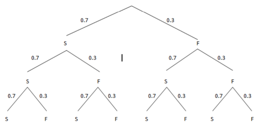
\(P(X=2)=P(S S F)+P(S F S)+P(F S S)=(3)(0.7)^{2}(0.3)^{1}=0.441\)

There is about a 44% chance that Draymond Green will make exactly two free throws in three trials.

To find the probability Draymond makes at least 2 free throws, we would have to also consider when he makes all three shots (SSS).

\(P(X \geq 2)=P(X=2)+P(X=3)=(3)(0.7)^{2}(0.3)^{1}+(3)(0.7)^{3}(0.3)^{0}=0.441+.343=.784\)

There is about a 78.4% chance that Draymond Green will make at least two free throws in three trials.

For larger sample sizes, tree diagrams are too tedious to use. There is a formula to find the probability of exactly x success in n trials:

\[P(x)={ }_{n} C_{x} p^{x}(1-p)^{n-x} \nonumber \]

The combination formula \({ }_{n} C_{x}=\dfrac{n !}{x !(n-x) !}\) means the number of ways x successes can occur out of n trials. This formula is also tedious to use, so we will rely on tables or technology to calculate binomial probabilities.

Here is a summary of the Binomial Distribution

Binomial Probability Distribution (parameters= \(n, p\))

\(n\)= number of independent trials (sample size)

Two possible outcomes (Success/Failure) or (Yes/No)

\(\mathbf{p} = P\)(yes/success) on one trial      

\(q = 1‐p = P\)(no/failure) on one trial

\(X\) = Number of Yes/Successes {0, 1, 2, ..., n}

\(\mu=n p\)

\(\sigma^{2}=n p(1-p)\)

\(\sigma=\sqrt{n p(1-p)}\)

\(P(x)={ }_{n} C_{x} p^{x}(1-p)^{n-x}\)

Example: Quality control

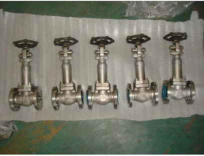
90% of super duplex globe vales valves⁶⁷ manufactured are good (not defective). A sample of 10 valves is selected. Define the random variable and determine the parameters.

Solution

\(X\) = number of good valves in the sample of 10.

\(n = 10, p = 0.9\)

Find the mean and variance

\(\mu=n p=(10)(0.9)=9\)

\(\sigma^{2}=n p(1-p)=(10)(0.9)(0.1)=0.9\)

For the following probability questions, we can use technology or a table. The displayed table was created by Minitab.

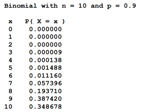
Find the probability of exactly 8 good valves being chosen.

\[P(X=8)=0.194 \nonumber \]

Find the probability of 9 or more good valves being chosen.

\[P(X \geq 9)=P(9)+P(10)=0.387+0.349=0.736\nonumber \]

Find the probability of 8 or fewer good valves being chosen.

\[P(X \leq 9)=P(0)+P(1)+\ldots+P(8) \nonumber \]  or instead use Rule of Complement and prior example

\[P(X \leq 9)=1-P(X \geq 9)=1-0.736=0.264 \nonumber \]