3.5: Working with Outliers

An outlier is a data point that is far removed from the other entries in the data set. Outliers could be caused by:

• Mistakes made in recording data
• Data that don’t belong in the population
• True rare events  

The first two cases are simple to deal with as we can correct errors or remove data that that does not belong in the population. The third case is more problematic as extreme outliers will increase the standard deviation dramatically and heavily skew the data.  

In The Black Swan, Nicholas Taleb argues that some populations with extreme outliers should not be analyzed with traditional confidence intervals and hypothesis testing.³⁰ He defines a Black Swan as an unpredictable extreme outlier that causes dramatic effects on the population. A recent example of a Black Swan was the catastrophic drop in the value of unregulated Credit Default Swap (CDS) real estate insurance investments which caused the near collapse of international banking system in 2008. The traditional statistical analysis that measured the risk of the CDS investments did not take into account the consequence of a rapid increase in the number of foreclosures of homes. In this case, statistics that measure investment performance and risk were useless and created a false sense of security for large banks and insurance companies.

Example: Realtor home sales

Here are the quarterly home sales for 10 realtors: 2   2   3   4   5   5   6   6   7   50

	With outlier	Without outlier
Mean	9.00	4.44
Median	5.00	5.00
Standard Deviation	14.51	1.81
Interquartile Range	3.00	3.50

In this example, the number 50 is an outlier. When calculating summary statistics, we can see that the mean and standard deviation are dramatically affected by the outlier, while the median and the interquartile range (which are based on the ranking of the data) are hardly changed. One solution when dealing with a population with extreme outliers is to use inferential statistics that use the ranks of the data, also called non‐parametric statistics.

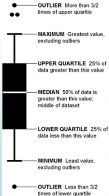
Using Box Plot to find outliers

• The “box” is the region between the 1st and 3rd quartiles.
• Possible outliers are more than 1.5 IQR’s from the box (inner fence)
• Probable outliers are more than 3 IQR’s from the box (outer fence)
• In the box plot below of the realtor example, the dotted lines represent the inner and outer “fences” that are 1.5 and 3 IQR’s respectively from the box. See how the data point 50 is well outside the outer fence and therefore an almost certain outlier.
• The whiskers now end at the most extreme value that is NOT a possible outlier.

Lower Inner Fence = Q1 – (1.5)IQR = 3 – (1.5)(3) = ‐1.5

Lower Outer Fence = Q1 – (3)IQR = 3 – (3)(3) = ‐6

Upper Inner Fence = Q3 + (1.5)IQR = 6 + (1.5)(3) = 10.5

Upper Outer Fence = Q3 + (3)IQR = 6 + (3)(3) = 15

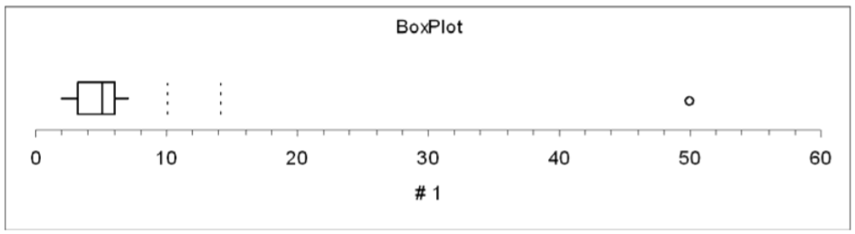
Since the value 50 is far beyond the outer fence of 15, 50 is an extreme outlier.

Steps for making a box plot (with outliers)

1. Draw the box between Q1 and Q3
2. Accurately plot the median
3. Determine possible outliers that are more than 1.5 interquartile ranges from the box.        

Lower Inner Fence = Q1 – (1.5)IQR          

Upper Inner Fence = Q3 + (1.5)IQR  

4. Mark outliers with a special character like a * or •.
5. Draw whiskers to minimum and maximum values that are not possible outliers.

(note: boxplot below not drawn to scale)

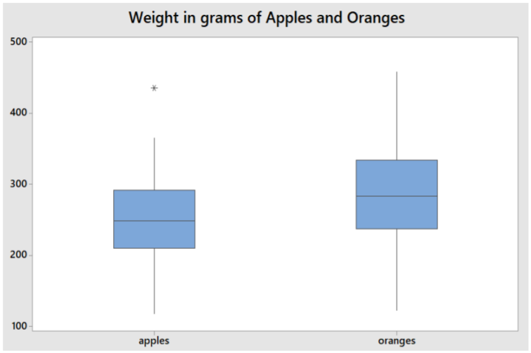
Example: Comparing apples to oranges

Using the summary statistics, make side‐by side box plots of the weights of 100 Fuji apples and 100 Navel oranges. Analyze and interpret the graphs, including outliers.

Summary Statistics:

Variable	Fruit	N	Minimum	Q1	Median	Q3	Maximum	IQR
weights	apples	100	118.00	210.00	248.00	291.50	435.00	81.50
	oranges	100	122.00	237.25	283.50	333.50	458.00	96.25

Solution

Oranges have a higher median weight compared to apples.

The IQR is slightly larger for oranges.

Both fruits have graphs that are mostly symmetric.

The apple that weighs 435 grams is a possible outlier since the weight exceeds the Inner Fence = 291.50 + 1.5(81.5) = 414.

The next highest apple weight is 365 grams.

Using the z‐score to find outliers

The z‐score can also be used to find outliers, but care must be taken since the mean and standard deviation are affected by outliers. One strategy is to remove the outlier before calculating these statistics.

Procedure for using z‐score to find outliers

1. Calculate the sample mean and standard deviation without the suspected outlier.
2. Calculate the Z‐score of the suspected outlier: \(z-\text { score }=\dfrac{X_{i}-\bar{X}}{s}\)
3. If the Z‐score is more than 3 or less than ‐3, that data point is a probable outlier.

Example: Realtor home sales

Determine if 50 is an outlier.

Solution

Determine the sample mean and standard deviation excluding the value 50.\[\bar{X}=4.44 \quad s=1.81 \nonumber \]

Determine the z‐score for 50.\[z-\text { score }=\dfrac{50-4.4}{1.81}=25.2 \nonumber \]

Since 25.2 is much greater than 3, the value 50 is an extreme outlier

Outliers, what to do?

There is no clear answer what to do about legitimate outliers. Do we remove them or leave them in?

For some populations, outliers don’t dramatically change the overall statistical analysis. Example: the tallest person in the world will not dramatically change the mean height of 10000 people.

However, for some populations, a single outlier will have a dramatic effect on statistical analysis (called “Black Swan” by Nicholas Taleb³¹), and inferential statistics may be invalid in analyzing these populations. Example: the richest person in the world will dramatically change the mean wealth of 10000 people.