3.3: Measures of Relative Standing

Last updated
Save as PDF

Page ID: 20840

\( \newcommand{\vecs}[1]{\overset { \scriptstyle \rightharpoonup} {\mathbf{#1}} } \) \( \newcommand{\vecd}[1]{\overset{-\!-\!\rightharpoonup}{\vphantom{a}\smash {#1}}} \)\(\newcommand{\id}{\mathrm{id}}\) \( \newcommand{\Span}{\mathrm{span}}\) \( \newcommand{\kernel}{\mathrm{null}\,}\) \( \newcommand{\range}{\mathrm{range}\,}\) \( \newcommand{\RealPart}{\mathrm{Re}}\) \( \newcommand{\ImaginaryPart}{\mathrm{Im}}\) \( \newcommand{\Argument}{\mathrm{Arg}}\) \( \newcommand{\norm}[1]{\| #1 \|}\) \( \newcommand{\inner}[2]{\langle #1, #2 \rangle}\) \( \newcommand{\Span}{\mathrm{span}}\) \(\newcommand{\id}{\mathrm{id}}\) \( \newcommand{\Span}{\mathrm{span}}\) \( \newcommand{\kernel}{\mathrm{null}\,}\) \( \newcommand{\range}{\mathrm{range}\,}\) \( \newcommand{\RealPart}{\mathrm{Re}}\) \( \newcommand{\ImaginaryPart}{\mathrm{Im}}\) \( \newcommand{\Argument}{\mathrm{Arg}}\) \( \newcommand{\norm}[1]{\| #1 \|}\) \( \newcommand{\inner}[2]{\langle #1, #2 \rangle}\) \( \newcommand{\Span}{\mathrm{span}}\)\(\newcommand{\AA}{\unicode[.8,0]{x212B}}\)

A student receives a score of 82 on a Midterm Exam and asks the instructor, “How well did I do on the test?” To answer this question, we need statistics that measure the ranking of this grade relative to the class. These statistics are called measure of relative standing.

The z‐score

Related to the Empirical Rule is the z‐score which measures how many standard deviations a particular data point is above or below the mean. Unusual observations would have a z‐score over 2 or under ‐2. Extreme observations would have z‐scores over 3 or under ‐3 and should be investigated as potential outliers. For a particular value from the data (\(X_{i}\)), we can easily calculate the z‐score for that value.

\[\text { Formula for z-score: } \quad z-\text { score }=\dfrac{X_{i}-\bar{X}}{s} \nonumber \]

For the student who received an 82 on the exam we can calculate the Z‐score if we know the sample mean and standard deviation for the class. Suppose for this class, the sample mean was 70 and the sample standard deviation was 10. Then for this student:

\[z-\text { score }=\dfrac{82-70}{10}=+1.2 \nonumber \]

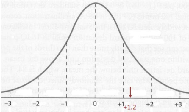
The z‐score of 1.7 tells us the student's score was well above average, but not highly unusual.

Interpreting z‐score for several students

Exam Score	z‐score	Interpretation
82	+1.2	well above average
66	-0.4	slightly below average
94	+2.4	unusually above average
34	-3.6	extremely below average

Example: Comparing apples to oranges

The sample mean for 100 Fuji apples was 252 grams and the standard deviation was 55 grams. The sample mean for 100 Navel oranges was 286 grams and the standard deviation was 67 grams. What would be more unusual: a small apple that weighed 130 grams or a large orange that weighed 430 grams?

Solution

Some people might say “The small apple is 122 grams below the mean and the large orange is 144 grams above the mean so the orange is more unusual”, but this does not take into account the spread of weights for apples and oranges. Instead, we should determine which z‐score is further from zero.

z‐score for apple = (130 – 252)/55 = ‐2.22

z‐score for orange = (430 – 286)/67 = +2.15

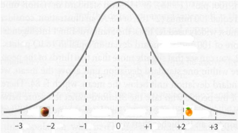
The small apple is slightly more unusual than the large orange because ‐2.22 is further from zero.

Percentile, Quartiles and the Interquartile Range

In an earlier section, we explored how we can use the ogive graph to calculate percentiles and quartiles for data. This section will introduce the percentile as a measure of relative standing.

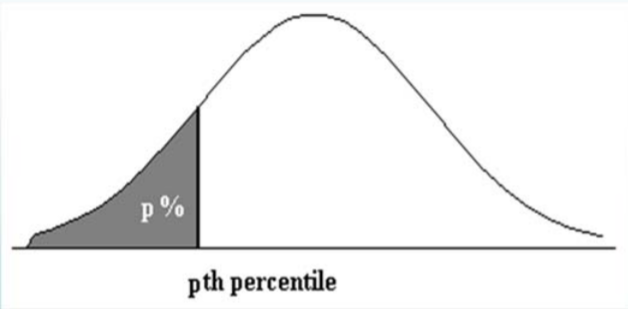
Definition: p^th Percentile

\(p^{th}\) Percentile ‐ the value of the data below which p percent of the data fall.

To calculate the location of the \(p^{th}\) percentile in a sample of size \(n\), use the formula:

\[p^{\text {th }} \text { percentile location }=p(n+1) \nonumber \]

The \(25^{th}\) percentile is also known as the 1st Quartile or Q1

The \(50^{th}\) percentile is also known as the 2nd Quartile or median

The \(75^{th}\) percentile is also known as the 3rd Quartile or Q3

Example: Students browsing the web

Let’s again return to the example of daily minutes spent on the internet by 30 students and use the empirical rule to find the 70th percentile.

Solution

Location of \(70^{th}\) percentile = 0.70(30+1) = 21.7 ≈ 22nd location

\(70^{th}\) percentile ≈ 107 minutes.

For a more accurate calculation, you can use linear interpolation of the fractional part of 21.7 by adding 30% of the 21st location to 70% of the 22nd location.

\(70^{th}\) percentile = (0.3)(105) + (0.7)(107) = 106.4 minutes

There is an alternative method to find the quartiles of data.

Find the median (2nd quartile). The median divides the data in half.
Q1 (1st quartile) will be the median of the first half of the data
Q3 (3rd quartile) will be the median of the second half of the data.

Example: Students browsing the web

Find the three quartiles for this data.

Solution

Median = (101 +102)/2 = 101.5

Q1 = 1st quartile = 87

Q3 = 3rd quartile = 108

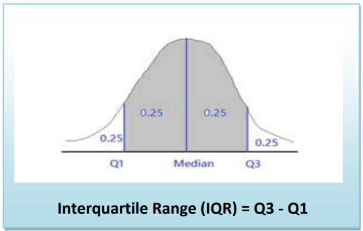
Interquartile Range

Definition: Interquartile Range (IQR)

A measure of variability based on the ranking of the data is called the Interquartile Range (IQR), which is the difference between the third quartile and the first quartile. The IQR represents the range of the middle 50% of the data and represents variability of the data with respect to the median.

Example: Students browsing the web

Find and explain the interquartile range for this data

Solution

IQR = 108 ‐87 = 21 minutes

The middle 50% of the observations are between 87 and 108 minutes.