5.2: Is there a difference? Comparing two samples

Two-sample Tests

Studying two samples, we use the same approach with two hypotheses. The typical null hypothesis is “there is no difference between these two samples”—in other words, they are both drawn from the same population. The alternative hypothesis is “there is a difference between these two samples”. There are many other ways to say that:

• Null: difference equal to 0 \(\approx\) samples similar \(\approx\) samples related \(\approx\) samples came from the same population
• Alternative: difference not equal to 0 \(\approx\) samples different \(\approx\) samples non-related \(\approx\) samples came from different populations

And, in terms of p-value:

If the data are “parametric”, then a parametric t-test is required. If the variables that we want to compare were obtained on different objects, we will use a two-sample t-test for independent variables, which is called with the command t.test():

Code \(\PageIndex{1}\) (R):

bpress <- read.table("data/bpress.txt", h=TRUE)
head(bpress)
drug.d <- bpress$DRUG.10 - bpress$DRUG.1
placebo.d <- bpress$PLACEBO.10 - bpress$PLACEBO.1
sapply(data.frame(placebo.d, drug.d), Normality) # asmisc.r
Normality <- function(a) {ifelse(shapiro.test(a)$p.value < 0.05, "NOT NORMAL", "NORMAL")}
t.test(placebo.d, drug.d)

There is a long output. Please note the following:

• Apart from the normality, there is a second assumption of the classic t-test, homogeneity of variances. However, R by default performs more complicated Welch test which does not require homogeneity. This is why degrees of freedom are not a whole number.
• t is a t statistic and df are degrees of freedom (related with number of cases), they both needed to calculate the p-value.
• Confidence interval is the second most important output of the R t.test(). It is recommended to supply confidence intervals and effect sizes (see below) wherever possible. If zero is within the confidence interval, there is a difference.
• p-value is small, therefore the probability to “raise the false alarm” when “nothing happens” is also small. Consequently, we reject the null hypothesis (“nothing happens”, “no difference”, “no effect”) and therefore switch to the alternative hypothesis (“there is a difference between drugs”.)

We can use the following order from most to least important:

1. p-value is first because it helps to make decision;
2. confidence interval;
3. t statistic;
4. degrees of freedom.

Results of t-test did not come out of nowhere. Let us calculate the same thing manually (actually, half-manually because we will use degrees of freedom from the above test results):

Code \(\PageIndex{2}\) (R):

bpress <- read.table("data/bpress.txt", h=TRUE)
drug.d <- bpress$DRUG.10 - bpress$DRUG.1
placebo.d <- bpress$PLACEBO.10 - bpress$PLACEBO.1
df <- 6.7586
v1 <- var(placebo.d)
v2 <- var(drug.d)
(t.stat <- (mean(placebo.d) - mean(drug.d))/sqrt(v1/5 + v2/5))
(p.value <- 2*pt(-abs(t.stat), df))

(Function pt() calculates values of the Student distribution, the one which is used for t-test. Actually, instead of direct calculation, this and similar functions estimate p-values using tables and approximate formulas. This is because the direct calculation of exact probability requires integration, determining the square under the curve, like \(\alpha\) from Figure 5.1.1.)

Using t statistic and degrees of freedom, one can calculate p-value without running test. This is why to report result of t-test (and related Wilcoxon test, see later), most researchers list statistic, degrees of freedom (for t-test only) and p-value.

Instead of “short form” from above, you can use a “long form” when the first column of the data frame contains all data, and the second indicates groups:

Code \(\PageIndex{3}\) (R):

bpress <- read.table("data/bpress.txt", h=TRUE)
drug.d <- bpress$DRUG.10 - bpress$DRUG.1
placebo.d <- bpress$PLACEBO.10 - bpress$PLACEBO.1
long <- stack(data.frame(placebo.d, drug.d))
head(long)
t.test(values ~ ind, data=long)

(Note the formula interface which usually comes together with a long form.)

Long form is handy also for plotting and data manipulations (check the plot yourself):

Code \(\PageIndex{4}\) (R):

bpress <- read.table("data/bpress.txt", h=TRUE)
drug.d <- bpress$DRUG.10 - bpress$DRUG.1
placebo.d <- bpress$PLACEBO.10 - bpress$PLACEBO.1
long <- stack(data.frame(placebo.d, drug.d))
boxplot(values ~ ind, data=long)
tapply(long$values, long$ind, sd)
aggregate(values ~ ind, range, data=long)

Another example of long form is the embedded beaver2 data:

Code \(\PageIndex{5}\) (R):

Normality <- function(a) {ifelse(shapiro.test(a)$p.value < 0.05, "NOT NORMAL", "NORMAL")}
tapply(beaver2$temp, beaver2$activ, Normality) # asmisc.r
boxplot(temp ~ activ, data=beaver2)
t.test(temp ~ activ, data=beaver2)

(Check the boxplot yourself. We assumed that temperature was measured randomly.)

Again, p-value is much less than 0.05, and we must reject the null hypothesis that temperatures are not different when beaver is active or not.

To convert long form into short, use unstack() function:

Code \(\PageIndex{6}\) (R):

uu <- unstack(beaver2, temp ~ activ)
str(uu)

(Note that result is a list because numbers of observations for active and inactive beaver are different. This is another plus of long form: it can handle subsets of unequal size.)

If measurements were obtained on one object, a paired t-test should be used. In fact, it is just one-sample t-test applied to differences between each pair of measurements. To do paired t-test in R, use the parameter paired=TRUE. It is not illegal to choose common t-test for paired data, but paired tests are usually more powerful:

Code \(\PageIndex{7}\) (R):

bpress <- read.table("data/bpress.txt", h=TRUE)
drug.d <- bpress$DRUG.10 - bpress$DRUG.1
placebo.d <- bpress$PLACEBO.10 - bpress$PLACEBO.1
sapply(bpress, Normality) # asmisc.r
Normality <- function(a) {ifelse(shapiro.test(a)$p.value < 0.05, "NOT NORMAL", "NORMAL")}
attach(bpress)
t.test(DRUG.1, DRUG.10, paired=TRUE)
t.test(DRUG.10 - DRUG.1, mu=0) # same results
t.test(DRUG.1, DRUG.10) # non-paired
detach(bpress)

If the case of blood pressure measurements, common t-test does not “know” which factor is responsible more for the differences: drug influence or individual variation between people. Paired t-test excludes individual variation and allows each person to serve as its own control, this is why it is more precise.

Also more precise (if the alternative hypothesis is correctly specified) are one-tailed tests:

Code \(\PageIndex{8}\) (R):

bpress <- read.table("data/bpress.txt", h=TRUE)
drug.d <- bpress$DRUG.10 - bpress$DRUG.1
placebo.d <- bpress$PLACEBO.10 - bpress$PLACEBO.1
attach(bpress)
t.test(PLACEBO.10, DRUG.10, alt="greater") # one-tailed test
t.test(PLACEBO.10, DRUG.10) # "common" test
detach(bpress)

(Here we used another alternative hypothesis: instead of guessing difference, we guessed that blood pressure in “placebo” group was greater on 10th day.)

Highly important note: all decisions related with the statistical tests (parametric or nonparametric, paired or non-paired, one-sided or two-sided, 0.05 or 0.01) must be done a priori, before the analysis. The “hunting for the p-value” is illegal!

If we work with nonparametric data, nonparametric Wilcoxon test (also known as a Mann-Whitney test) is required, under the command wilcox.test():

Code \(\PageIndex{9}\) (R):

Normality <- function(a) {ifelse(shapiro.test(a)$p.value < 0.05, "NOT NORMAL", "NORMAL")}
tapply(ToothGrowth$len, ToothGrowth$supp, Normality) # asmisc.r
boxplot(len ~ supp, data=ToothGrowth, notch=TRUE)
wilcox.test(len ~ supp, data=ToothGrowth)

(Please run the boxplot code and note the use of notches. It is commonly accepted that overlapping notches is a sign of no difference. And yes, Wilcoxon test supports that. Notches are not default because in many cases, boxplots are visually not overlapped. By the way, we assumed here that only supp variable is present and ignored dose (see ?ToothGrowth for more details).)

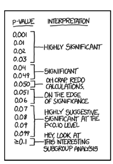
And yes, it is really tempting to conclude something except “stay with null” if p-value is 0.06 (Figure \(\PageIndex{1}\)) but no. This is not allowed.

Like in the t-test, paired data requires the parameter paired=TRUE:

Code \(\PageIndex{10}\) (R):

Normality <- function(a) {ifelse(shapiro.test(a)$p.value < 0.05, "NOT NORMAL", "NORMAL")}
w0 <- ChickWeight$weight[ChickWeight$Time == 0]
w2 <- ChickWeight$weight[ChickWeight$Time == 2]
sapply(data.frame(w0, w2), Normality)
boxplot(w0, w2)
wilcox.test(w0, w2, paired=TRUE)

(Chicken weights are really different between hatching and second day! Please check the boxplot yourself.)

Figure \(\PageIndex{1}\) How not to interpret p-values (taken from XKCD, https://xkcd.com/1478/)

Nonparametric tests are generally more universal since they do not assume any particular distribution. However, they are less powerful (prone to Type II error, “carelessness”). Moreover, nonparametric tests based on ranks (like Wilcoxon test) are sensitive to the heterogeneity of variances\(^{[1]}\). All in all, parametric tests are preferable when data comply with their assumptions. Table \(\PageIndex{1}\) summarizes this simple procedure.

Table \(\PageIndex{1}\): How to choose two-sample test in R. This table should be read from the top right cell.

	Paired: one object, two measures	Non-paired
Normal	t.test(..., paired=TRUE)	t.test(...)
Non-normal	wilcox.test(..., paired=TRUE)	wilcox.test(...)

Embedded in R is the classic data set used in the original work of Student (the pseudonym of mathematician William Sealy Gossett who worked for Guinness brewery and was not allowed to use his real name for publications). This work was concerned with comparing the effects of two drugs on the duration of sleep for 10 patients.

In R these data are available under the name sleep (Figure \(\PageIndex{2}\) shows corresponding boxplots). The data is in the long form: column extra contains the increase of the sleep times (in hours, positive or negative) while the column group indicates the group (type of drug).

Code \(\PageIndex{11}\) (R):

plot(extra ~ group, data=sleep)

Figure \(\PageIndex{2}\) The average increase of the sleep with two drugs.

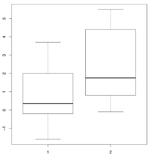
(Plotting uses the “model formula”: in this case, extra ~ group. R is smart enough to understand that group is the “splitting” factor and should be used to make two boxplots.)

The effect of each drug on each person is individual, but the average length by which the drug prolongs sleep can be considered a reasonable representation of the “strength” of the drug. With this assumption, we will attempt to use a two sample test to determine whether there is a significant difference between the means of the two samples corresponding to the two drugs. First, we need to determine which test to use:

Code \(\PageIndex{12}\) (R):

Normality <- function(a) {ifelse(shapiro.test(a)$p.value < 0.05, "NOT NORMAL", "NORMAL")}
tapply(sleep$extra, sleep$group, Normality) # asmisc.r

(Data in the long form is perfectly suitable for tapply() which splits first argument in accordance with second, and then apply the third argument to all subsets.)

Since the data comply with the normality assumption, we can now employ parametric paired t-test:

Code \(\PageIndex{13}\) (R):

t.test(extra ~ group, data=sleep, paired=TRUE)

(Yes, we should reject null hypothesis about no difference.)

How about the probability of Type II errors (false negatives)? It is related with statistical power, and could be calculated through power test:

Code \(\PageIndex{14}\) (R):

power.t.test(n=10, sig.level=0.05, d=1.58)

Therefore, if we want the level of significance 0.05, sample size 10 and the effect (difference between means) 1.58, then probability of false negatives should be approximately \(1-0.92=0.08\) which is really low. Altogether, this makes close to 100% our positive predictive value (PPV), probability of our positive result (observed difference) to be truly positive for the whole statistical population. Package caret is able to calculate PPV and other values related with statistical power.

It is sometimes said that t-test can handle the number of samples as low as just four. This is not absolutely correct since the power is suffering from small sample sizes, but it is true that main reason to invent t-test was to work with small samples, smaller then “rule of 30” discussed in first chapter.

Both t-test and Wilcoxon test check for differences only between measures of central tendency (for example, means). These homogeneous samples

Code \(\PageIndex{15}\) (R):

(aa <- 1:9)
(bb <- rep(5, 9))

have the same mean but different variances (check it yourself), and thus the difference would not be detected with t-test or Wilcoxon test. Of course, tests for scale measures (like var.test()) also exist, and they might find the difference. You might try them yourself. The third homogeneous sample complements the case:

Code \(\PageIndex{16}\) (R):

(xx <- 51:59)

as differences in centers, not in ranges, will now be detected (check it).

There are many other two sample tests. One of these, the sign test, is so simple that it does not exist in R by default. The sign test first calculates differences between every pair of elements in two samples of equal size (it is a paired test). Then, it considers only the positive values and disregards others. The idea is that if samples were taken from the same distribution, then approximately half the differences should be positive, and the proportions test will not find a significant difference between 50% and the proportion of positive differences. If the samples are different, then the proportion of positive differences should be significantly more or less than half.

Come up with R code to carry out sign test, and test two samples that were mentioned at the beginning of the section.

The standard data set airquality contains information about the amount of ozone in the atmosphere around New York City from May to September 1973. The concentration of ozone is presented as a rounded mean for every day. To analyze it conservatively, we use nonparametric methods.

Determine how close to normally distributed the monthly concentration measurements are.

Let us test the hypothesis that ozone levels in May and August were the same:

Code \(\PageIndex{17}\) (R):

wilcox.test(Ozone ~ Month, data=airquality, subset = Month %in% c(5, 8), conf.int=TRUE)

(Since Month is a discrete variable as the “number” simply represents the month, the values of Ozone will be grouped by month. We used the parameter subset with the operator %in%, which chooses May and August, the 5th and 8th month. To obtain the confidence interval, we used the additional parameter conf.int. \(W\) is the statistic employed in the calculation of p-values. Finally, there were warning messages about ties which we ignored.)

The test rejects the null hypothesis, of equality between the distribution of ozone concentrations in May and August, fairly confidently. This is plausible because the ozone level in the atmosphere strongly depends on solar activity, temperature and wind.

Differences between samples are well represented by box plots (Figure \(\PageIndex{3}\)):

Code \(\PageIndex{18}\) (R):

boxplot(Ozone ~ Month, data=airquality, subset=Month %in% c(5, 8), notch=TRUE)

Figure \(\PageIndex{3}\) Distribution of ozone in May and June.

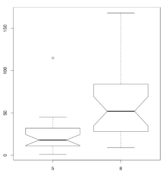
(Note that in the boxplot() command we use the same formula as the statistical model. Option subset is alternative way to select from data frame.)

It is conventionally considered that if the boxes overlap by more than a third of their length, the samples are not significantly different.

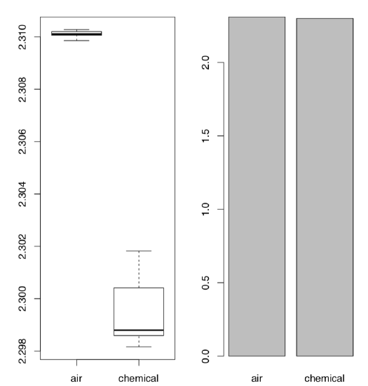
The last example in this section is related with the discovery of argon. At first, there was no understanding that inert gases exist in nature as they are really hard to discover chemically. But in the end of XIX century, data start to accumulate that something is wrong with nitrogen gas (N\(_2\)). Physicist Lord Rayleigh presented data which show that densities of nitrogen gas produced from ammonia and nitrogen gas produced from air are different:

Code \(\PageIndex{19}\) (R):

ar <- read.table("data/argon.txt")
unstack(ar, form=V2 ~ V1)

As one might see, the difference is really small. However, it was enough for chemist Sir William Ramsay to accept it as a challenge. Both scientists performed series of advanced experiments which finally resulted in the discovery of new gas, argon. In 1904, they received two Nobel Prizes, one in physical science and one in chemistry. From the statistical point of view, most striking is how the visualization methods perform with this data:

Code \(\PageIndex{20}\) (R):

ar <- read.table("data/argon.txt")
means <- tapply(ar$V2, ar$V1, mean, na.rm=TRUE)
oldpar <- par(mfrow=1:2)
boxplot(V2 ~ V1, data=ar)
barplot(means)
par(oldpar)

The Figure \(\PageIndex{4}\) shows as clear as possible that boxplots have great advantage over traditional barplots, especially in cases of two-sample comparison.

We recommend therefore to avoid barplots, and by all means avoid so-called “dynamite plots” (barplots with error bars on tops). Beware of dynamite!

Their most important disadvantages are (1) they hide primary data (so they are not exploratory), and in the same time, do not illustrate any statistical test (so they are not inferential); (2) they (frequently wrongly) assume that data is symmetric and parametric; (3) they use space inefficiently, have low data-to-ink ratio; (4) they cause an optical illusion in which the reader adds some of the error bar to the height of the main bar when trying to judge the heights of the main bars; (5) the standard deviation error bar (typical there) has no direct relation even with comparing two samples (see above how t-test works), and has almost nothing to do with comparison of multiple samples (see below how ANOVA works). And, of course, they do not help Lord Rayleigh and Sir William Ramsay to receive their Nobel prizes.

Figure \(\PageIndex{4}\) Which of these two plots would help Lord Rayleigh and Sir William Ramsay more to receive their Nobel Prizes? (The idea from Tukey, 1977.)

Please check the Lord Rayleigh data with the appropriate statistical test and report results.

So what to do with dynamite plots? Replace them with boxplots. The only disadvantage of boxplots is that they are harder to draw with hand which sounds funny in the era of computers. This, by the way, explains partly why there are so many dynamite around: they are sort of legacy pre-computer times.

A supermarket has two cashiers. To analyze their work efficiency, the length of the line at each of their registers is recorded several times a day. The data are recorded in kass.txt. Which cashier processes customers more quickly?

Effect sizes

Statistical tests allow to make decisions but do not show how different are samples. Consider the following examples:

Code \(\PageIndex{21}\) (R):

wilcox.test(1:10, 1:10 + 0.001, paired=TRUE)
wilcox.test(1:10, 1:10 + 0.0001, paired=TRUE)

(Here difference decreases but p-value does not grow!)

One of the beginner’s mistakes is to think that p-values measure differences, but this is really wrong.

P-values are probabilities and are not supposed to measure anything. They could be used only in one, binary, yes/no way: to help with statistical decisions.

In addition, the researcher can almost always obtain a reasonably good p-value, even if effect is minuscule, like in the second example above.

To estimate the extent of differences between populations, effect sizes were invented. They are strongly recommended to report together with p-values.

Package effsize calculates several effect size metrics and provides interpretations of their magnitude.

Cohen’s d is the parametric effect size metric which indicates difference between two means:

Code \(\PageIndex{22}\) (R):

library(effsize)
cohen.d(extra ~ group, data=sleep)

(Note that in the last example, effect size is large with confidence interval including zero; this spoils the “large” effect.)

If the data is nonparametric, it is better to use Cliff’s Delta:

Code \(\PageIndex{23}\) (R):

cliff.delta(1:10, 1:10+0.001)
cliff.delta(Ozone ~ Month, data=airquality, subset = Month %in% c(5, 8))

Now we have quite a few measurements to keep in memory. The simple table below emphasizes most frequently used ones:

	Center	Scale	Test	Effect
Parametric	Mean	Standard deviation	t-test	Cohen’s D
Non-parametric	Median	IQR, MAD	Wilcoxon test	Cliff’s Delta

Table \(\PageIndex{2}\): Most frequently used numerical tools, both for one and two samples.

There are many measures of effect sizes. In biology, useful is coefficient of divergence (\(K\)) discovered by Alexander Lyubishchev in 1959, and related with the recently introduced squared strictly standardized mean difference (SSSMD):

Code \(\PageIndex{24}\) (R):

K(extra ~ group, data=sleep) # asmisc.r
summary(K(extra ~ group, data=sleep))

Lyubishchev noted that good biological species should have \(K>18\), this means no transgression.

Coefficient of divergence is robust to allometric changes:

Code \(\PageIndex{25}\) (R):

K(extra ~ group, data=sleep) # asmisc.r
(aa <- 1:9)
summary(K(aa*3, aa*10)) # asmisc.r
cliff.delta(1:10, 1:10+0.001)
cliff.delta(Ozone ~ Month, data=airquality, subset = Month %in% c(5, 8))
cliff.delta(aa*3, aa*10)

There is also MAD-based nonparametric variant of \(K\):

Code \(\PageIndex{26}\) (R):

K(extra ~ group, data=sleep) # asmisc.r
summary(K(1:10, 1:10+0.001, mad=TRUE)) # asmisc.r
(dd <- K(Ozone ~ Month, data=airquality[airquality$Month %in% c(5, 8), ], mad=TRUE)) # asmisc.r
summary(dd)

In the data file grades.txt are the grades of a particular group of students for the first exam (in the column labeled A1) and the second exam (A2), as well as the grades of a second group of students for the first exam (B1). Do the A class grades for the first and second exams differ? Which class did better in the first exam, A or B? Report significances, confidence intervals and effect sizes.

In the open repository, file aegopodium.txt contains measurements of leaves of sun and shade Aegopodium podagraria (ground elder) plants. Please find the character which is most different between sun and shade and apply the appropriate statistical test to find if this difference is significant. Report also the confidence interval and effect size.

References

1. There is a workaround though, robust rank order test, look for the function Rro.test() in theasmisc.r.