5.1: What is a statistical test?

Suppose that we compared two sets of numbers, measurements which came from two samples. From comparison, we found that they are different. But how to know if this difference did not arise by chance? In other words, how to decide that our two samples are truly different, i.e. did not come from the one population?

These samples could be, for example, measurements of systolic blood pressure. If we study the drug which potentially lowers the blood pressure, it is sensible to mix it randomly with a placebo, and then ask members of the group to report their blood pressure on the first day of trial and, saying, on the tenth day. Then the difference between two measurements will allow to decide if there is any effect:

Code \(\PageIndex{1}\) (R):

bpress <- read.table("data/bpress.txt", h=TRUE)
head(bpress)
drug.d <- bpress$DRUG.10 - bpress$DRUG.1
placebo.d <- bpress$PLACEBO.10 - bpress$PLACEBO.1
mean(drug.d - placebo.d)
boxplot(bpress)

Now, there is a promising effect, sufficient difference between blood pressure differences with drug and with placebo. This is also visible well with boxplots (check it yourself). How to test it? We already know how to use p-value, but it is the end of logical chain. Let us start from the beginning.

Statistical hypotheses

Philosophers postulated that science can never prove a theory, but only disprove it. If we collect 1000 facts that support a theory, it does not mean we have proved it—it is possible that the 1001st piece of evidence will disprove it. This is why in statistical testing we commonly use two hypotheses. The one we are trying to prove is called the alternative hypothesis (\(H_1\)). The other, default one, is called the null hypothesis (\(H_0\)). The null hypothesis is a proposition of absence of something (for example, difference between two samples or relationship between two variables). We cannot prove the alternative hypothesis, but we can reject the null hypothesis and therefore switch to the alternative. If we cannot reject the null hypothesis, then we must stay with it.

Statistical errors

With two hypotheses, there are four possible outcomes (Table \(\PageIndex{1}\)).

The first (a) and the last (d) outcomes are ideal cases: we either accept the null hypothesis which is correct for the population studied, or we reject \(H_0\) when it is wrong.

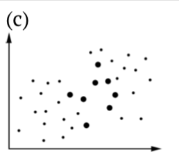
If we have accepted the alternative hypothesis, when it is not true, we have committed a Type I statistical error—we have found a pattern that does not exist. This situation is often called “false positive”, or “false alarm”. The probability of committing a Type I error is connected with a p-value which is always reported as one of results of a statistical test. In fact, p-value is a probability to have same or greater effect if the null hypothesis is true.

Imagine security officer on the night duty who hears something strange. There are two choices: jump and check if this noise is an indication of something important, or continue to relax. If the noise outside is not important or even not real but officer jumped, this is the Type I error. The probability to hear the suspicious noise when actually nothing happens in a p-value.

sample\population	Null is true	Alternative is true
Accept null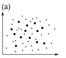
Accept alternative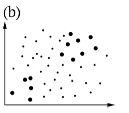

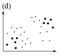Table \(\PageIndex{1}\) Statistical hypotheses, including illustrations of (b) Type I and (c) Type II errors. Bigger dots are samples, all dots are population(s).

For the security officer, it is probably better to commit Type I error than to skip something important. However, in science the situation is opposite: we always stay with the \(H_0\) when the probability of committing a Type I error is too high. Philosophically, this is a variant of Occam’s razor: scientists always prefer not to introduce anything (i.e., switch to alternative) without necessity.

the man who single-handedly saved the world from nuclear war

This approach could be found also in other spheres of our life. Read the Wikipedia article about Stanislav Petrov (https://en.Wikipedia.org/wiki/Stanislav_Petrov); this is another example when false alarm is too costly.

The obvious question is what probability is “too high”? The conventional answer places that threshold at 0.05—the alternative hypothesis is accepted if the p-value is less than 5% (more than 95% confidence level). In medicine, with human lives as stake, the thresholds are set even more strictly, at 1% or even 0.1%. Contrary, in social sciences, it is frequent to accept 10% as a threshold. Whatever was chosen as a threshold, it must be set a priori, before any test. It is not allowed to modify threshold in order to find an excuse for statistical decision in mind.

Figure \(\PageIndex{1}\) Scheme of statistical decision (for 1-tailed test). \(\alpha\) is the probability of Type I error, \(\beta\)—of Type II error. Before the test, we must set \(\alpha\), usually to 0.05. Then we use original data to calculate statistic (guess location of black vertical line). Next, we use statistic to calculate p-value. Finally, if p-value is less then \(\alpha\), we reject the null hypothesis.

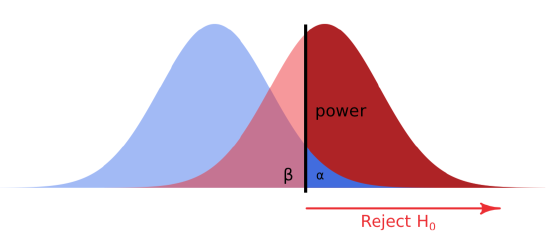
Accept the null hypothesis when in fact the alternative is true is a Type II statistical error—failure to detect a pattern that actually exists. This is called “false negative”, “carelessness”. If the careless security officer did not jump when the noise outside is really important, this is Type II error. Probability of committing type II error is expressed as power of the statistical test (Figure \(\PageIndex{1}\)). The smaller is this probability, the more powerful is the test.