6.3: Probability of the success- logistic regression

There are a few analytical methods working with categorical variables. Practically, we are restricted here with proportion tests and chi-squared. However, the goal sometimes is more complicated as we may want to check not only the presence of the correspondence but also its features—something like regression analysis but for the nominal data. In formula language, this might be described as

factor ~ influence

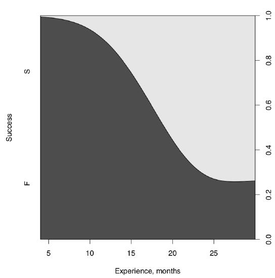
Below is an example using data from hiring interviews. Programmers with different months of professional experience were asked to write a program on paper. Then the program was entered into the memory of a computer and if it worked, the case was marked with “S” (success) and “F” (failure) otherwise:

Code \(\PageIndex{1}\) (R):

l <- read.table("data/logit.txt")
head(l)

Figure \(\PageIndex{1}\) TukeyHSD() plot for supplement-dose multiple comparisons (ToothGrowth data).

It is more or less obvious more experienced programmers are more successful. This is even possible to check visually, with cdplot() (Figure \(\PageIndex{2}\)):

Code \(\PageIndex{2}\) (R):

l <- read.table("data/logit.txt")
cdplot(V2 ~ V1, data=l, xlab="Experience, months", ylab="Success")

But is it possible to determine numerically the dependence between years of experience and programming success? Contingency tables is not a good solution because V1 is a measurement variable. Linear regression will not work because the response here is a factor. But there is a solution. We can research the model where the response is not a success/failure but the probability of success (which, as all probabilities is a measurement variable changing from 0 to 1):

Code \(\PageIndex{3}\) (R):

l <- read.table("data/logit.txt")
l.logit <- glm(V2 ~ V1, family=binomial, data=l)
summary(l.logit)

Figure \(\PageIndex{1}\) Conditional density plot shows the probability of programmer’s success.

Not going deeply into details, we can see here that both parameters of the regression are significant since p-values are small. This is enough to say that the experience influences the programming success.

The file seeing.txt came from the results of the following experiment. People were demonstrated some objects for the short time, and later they were asked to describe these objects. First column of the data file contains the person ID, second—the number of object (five objects were shown to each person in sequence) and the third column is the success/failure of description (in binary 0/1 format). Is there dependence between the object number and the success?

The output of summary.glm() contains the AIC value. It is accepted that smaller AIC corresponds with the more optimal model. To show it, we will return to the intoxication example from the previous chapter. Tomatoes or salad?

Code \(\PageIndex{4}\) (R):

tox <- read.table("data/poisoning.txt", h=TRUE)
tox.logit <- glm(formula=I(2-ILL) ~ CAESAR + TOMATO, family=binomial, data=tox)
tox.logit2 <- update(tox.logit, . ~ . - TOMATO)
tox.logit3 <- update(tox.logit, . ~ . - CAESAR)

At first, we created the logistic regression model. Since it “needs” the binary response, we subtracted the ILL value from 2 so the illness became encoded as 0 and no illness as 1. I() function was used to avoid the subtraction to be interpret as a model formula, and our minus symbol had only arithmetical meaning. On the next step, we used update() to modify the starting model removing tomatoes, then we removed the salad (dots mean that we use all initial influences and responses). Now to the AIC:

Code \(\PageIndex{5}\) (R):

tox <- read.table("data/poisoning.txt", h=TRUE)
tox.logit <- glm(formula=I(2-ILL) ~ CAESAR + TOMATO, family=binomial, data=tox)
tox.logit2 <- update(tox.logit, . ~ . - TOMATO)
tox.logit3 <- update(tox.logit, . ~ . - CAESAR)
tox.logit$aic
tox.logit2$aic
tox.logit3$aic

The model without tomatoes but with salad is the most optimal. It means that the poisoning agent was most likely the Caesar salad alone.

Now, for the sake of completeness, readers might have question if there are methods similar to logistic regression but using not two but many factor levels as response? And methods using ranked (ordinal) variables as response? (As a reminder, measurement variable as a response is a property of linear regression and similar.) Their names are multinomial regression and ordinal regression, and appropriate functions exist in several R packages, e.g., nnet, rms and ordinal.

File juniperus.txt in the open repository contains measurements of morphological and ecological characters in several Arctic populations of junipers (Juniperus). Please analyze how measurements are distributed among populations, and check specifically if the needle length is different between locations.

Another problem is that junipers of smaller size (height less than 1 m) and with shorter needles (less than 8 mm) were frequently separated from the common juniper (Juniperus communis) into another species, J. sibirica. Please check if plants with J. sibirica characters present in data, and does the probability of being J. sibirica depends on the amount of shading pine trees in vicinity (character PINE.N).