
6.5: Sampling Distribution and the Central Limit Theorem
- Page ID
- 5196

You now have most of the skills to start statistical inference, but you need one more concept.
First, it would be helpful to state what statistical inference is in more accurate terms.
Definition \(\PageIndex{1}\):Statistical Inference
Statistical Inference: to make accurate decisions about parameters from statistics.
When it says “accurate decision,” you want to be able to measure how accurate. You measure how accurate using probability. In both binomial and normal distributions, you needed to know that the random variable followed either distribution. You need to know how the statistic is distributed and then you can find probabilities. In other words, you need to know the shape of the sample mean or whatever statistic you want to make a decision about.
How is the statistic distributed? This is answered with a sampling distribution.
Definition \(\PageIndex{2}\): Sampling Distribution
Sampling Distribution: how a sample statistic is distributed when repeated trials of size n are taken.
Example \(\PageIndex{1}\) sampling distribution
Suppose you throw a penny and count how often a head comes up. The random variable is x = number of heads. The probability distribution (pdf) of this random variable is presented in Figure \(\PageIndex{1}\).
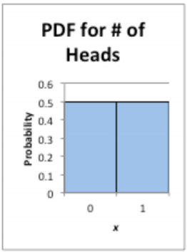.png?revision=1)
Solution
Repeat this experiment 10 times, which means n = 10. Here is the data set:
{1, 1, 1, 1, 0, 0, 0, 0, 0, 0}. The mean of this sample is 0.4. Now take another sample. Here is that data set:
{1, 1, 1, 0, 1, 0, 1, 1, 0, 0}. The mean of this sample is 0.6. Another sample looks like:
{0, 1, 0, 1, 1, 1, 1, 1, 0, 1}. The mean of this sample is 0.7. Repeat this 40 times. You could get these means:
| 0.4 | 0.6 | 0.7 | 0.3 | 0.3 | 0.2 | 0.5 | 0.5 | 0.5 | 0.5 |
| 0.4 | 0.4 | 0.5 | 0.7 | 0.7 | 0.6 | 0.4 | 0.4 | 0.4 | 0.6 |
| 0.7 | 0.7 | 0.3 | 0.5 | 0.6 | 0.3 | 0.3 | 0.8 | 0.3 | 0.6 |
| 0.4 | 0.3 | 0.5 | 0.6 | 0.5 | 0.6 | 0.3 | 0.5 | 0.6 | 0.2 |
Example \(\PageIndex{2}\) contains the distribution of these sample means (just count how many of each number there are and then divide by 40 to obtain the relative frequency).
| Sample Mean | Probability |
|---|---|
| 0.1 | 0 |
| 0.2 | 0.05 |
| 0.3 | 0.2 |
| 0.4 | 0.175 |
| 0.5 | 0.225 |
| 0.6 | 0.2 |
| 0.7 | 0.125 |
| 0.8 | 0.025 |
| 0.9 | 0 |
Figure \(\PageIndex{2}\) contains the histogram of these sample means.
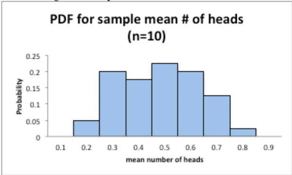.png?revision=1)
This distribution (represented graphically by the histogram) is a sampling distribution. That is all a sampling distribution is. It is a distribution created from statistics.
Notice the histogram does not look anything like the histogram of the original random variable. It also doesn’t look anything like a normal distribution, which is the only one you really know how to find probabilities. Granted you have the binomial, but the normal is better.
What does this distribution look like if instead of repeating the experiment 10 times you repeat it 20 times instead?
Example \(\PageIndex{3}\) contains 40 means when the experiment of flipping the coin is repeated 20 times.
| 0.5 | 0.45 | 0.7 | 0.55 | 0.65 | 0.6 | 0.4 | 0.35 | 0.45 | 0.6 |
| 0.5 | 0.5 | 0.65 | 0.5 | 0.5 | 0.35 | 0.55 | 0.4 | 0.65 | 0.3 |
| 0.4 | 0.5 | 0.45 | 0.45 | 0.65 | 0.7 | 0.6 | 0.5 | 0.7 | 0.7 |
| 0.7 | 0.45 | 0.35 | 0.6 | 0.65 | 0.55 | 0.35 | 0.4 | 0.55 | 0.6 |
Example \(\PageIndex{3}\) contains the sampling distribution of the sample means.
| Mean | Probability |
|---|---|
| 0.1 | 0 |
| 0.2 | 0 |
| 0.3 | 0.125 |
| 0.4 | 0.2 |
| 0.5 | 0.3 |
| 0.6 | 0.25 |
| 0.7 | 0.125 |
| 0.8 | 0 |
| 0.9 | 0 |
This histogram of the sampling distribution is displayed in Figure \(\PageIndex{3}\).
.png?revision=1)
Notice this histogram of the sample mean looks approximately symmetrical and could almost be called normal. What if you keep increasing n? What will the sampling distribution of the sample mean look like? In other words, what does the sampling distribution of \(\overline{x}\) look like as n gets even larger?
This depends on how the original distribution is distributed. In Example \(\PageIndex{1}\), the random variable was uniform looking. But as n increased to 20, the distribution of the mean looked approximately normal. What if the original distribution was normal? How big would n have to be? Before that question is answered, another concept is needed.
Note
Suppose you have a random variable that has a population mean, \(\mu\), and a population standard deviation, \(\sigma\). If a sample of size n is taken, then the sample mean, \(\overline{x}\) has a mean \(\mu_{\overline{x}}=\mu\) and standard deviation of \(\sigma_{\overline{x}}=\dfrac{\sigma}{\sqrt{n}}\). The standard deviation of \(\overline{x}\) is lower because by taking the mean you are averaging out the extreme values, which makes the distribution of the original random variable spread out.
You now know the center and the variability of \(\overline{x}\). You also want to know the shape of the distribution of \(\overline{x}\). You hope it is normal, since you know how to find probabilities using the normal curve. The following theorem tells you the requirement to have \(\overline{x}\) normally distributed.
Theorem \(\PageIndex{1}\) central limit theorem
Suppose a random variable is from any distribution. If a sample of size n is taken, then the sample mean, \(\overline{x}\), becomes normally distributed as n increases.
What this says is that no matter what x looks like, \(\overline{x}\) would look normal if n is large enough. Now, what size of n is large enough? That depends on how x is distributed in the first place. If the original random variable is normally distributed, then n just needs to be 2 or more data points. If the original random variable is somewhat mound shaped and symmetrical, then n needs to be greater than or equal to 30. Sometimes the sample size can be smaller, but this is a good rule of thumb. The sample size may have to be much larger if the original random variable is really skewed one way or another.
Now that you know when the sample mean will look like a normal distribution, then you can find the probability related to the sample mean. Remember that the mean of the sample mean is just the mean of the original data (\(\mu_{\overline{x}}=\mu\) ), but the standard deviation of the sample mean, \(\sigma_{\overline{x}}\), also known as the standard error of the mean, is actually \(\sigma_{\overline{x}}=\dfrac{\sigma}{\sqrt{n}}\). Make sure you use this in all calculations. If you are using the z-score, the formula when working with \(\overline{x}\) is \(z=\dfrac{\overline{x}-\mu_{\overline{x}}}{\sigma_{\overline{x}}}=\dfrac{\overline{x}-\mu}{\sigma / \sqrt{n}}\). If you are using the TI-83/84 calculator, then the input would be normalcdf(lower limit, upper limit, \(\mu\), \(\sigma / \sqrt{n}\) ). If you are using R, then the input would be pnorm( \(\overline{x}, \mu, \sigma / \operatorname{sqrt}(n) \)) to find the area to the left of \(\overline{x}\). Remember to subtract pnorm( \(\overline{x}, \mu, \sigma / \operatorname{sqrt}(n))\) ) from 1 if you want the area to the right of \(\overline{x}\).
Example \(\PageIndex{2}\) Finding probabilities for sample means
The birth weight of boy babies of European descent who were delivered at 40 weeks is normally distributed with a mean of 3687.6 g with a standard deviation of 410.5 g (Janssen, Thiessen, Klein, Whitfield, MacNab & Cullis-Kuhl, 2007). Suppose there were nine European descent boy babies born on a given day and the mean birth weight is calculated.
- State the random variable.
- What is the mean of the sample mean?
- What is the standard deviation of the sample mean?
- What distribution is the sample mean distributed as?
- Find the probability that the mean weight of the nine boy babies born was less than 3500.4 g.
- Find the probability that the mean weight of the nine babies born was less than 3452.5 g.
Solution
a. x = birth weight of boy babies (Note: the random variable is something you measure, and it is not the mean birth weight. Mean birth weight is calculated.)
b. \(\mu_{\overline{x}}=\mu=3687.6 \mathrm{g}\)
c. \(\sigma_{\overline{x}}=\dfrac{\sigma}{\sqrt{n}}=\dfrac{410.5}{\sqrt{9}}=\dfrac{410.5}{3} \approx 136.8 \mathrm{g}\)
d. Since the original random variable is distributed normally, then the sample mean is distributed normally.
e. You are looking for the \(P(\overline{x}<3500.4)\). You use the normalcdf command on the calculator. Remember to use the standard deviation you found in part c. However to reduce rounding error, type the division into the command. On the TI-83/84 you would have
\(P(\overline{x}<3500.4)=\text { normalcdf }(-1 E 99,3500.4,3687.6,410.5 \div \sqrt{9}) \approx 0.086\)
On R you would have
\(P(\overline{x}<3500.4)=\text { pnorm }(3500.4,3687.6,410.5 / s q r(9)) \approx 0.086\)
There is an 8.6% chance that the mean birth weight of the nine boy babies born would be less than 3500.4 g. Since this is more than 5%, this is not unusual.
f. You are looking for the \(P(\overline{x}<3452.5)\).
On TI-83/84:
\(P(\overline{x}<3452.5)=\text { normalcdf }(-1 E 99,3452.5,3687.6,410.5 \div \sqrt{9}) \approx 0.043\)
On R:
\(P(\overline{x}<3452.5)=\text { pnorm }(3452.5,3687.6,410.5 \div \sqrt{9}) \approx 0.043\)
There is a 4.3% chance that the mean birth weight of the nine boy babies born would be less than 3452.5 g. Since this is less than 5%, this would be an unusual event. If it actually happened, then you may think there is something unusual about this sample. Maybe some of the nine babies were born as multiples, which brings the mean weight down, or some or all of the babies were not of European descent (in fact the mean weight of South Asian boy babies is 3452.5 g), or some were born before 40 weeks, or the babies were born at high altitudes.
Example \(\PageIndex{3}\) finding probabilities for sample means
The age that American females first have intercourse is on average 17.4 years, with a standard deviation of approximately 2 years ("The Kinsey institute," 2013). This random variable is not normally distributed, though it is somewhat mound shaped.
- State the random variable.
- Suppose a sample of 35 American females is taken. Find the probability that the mean age that these 35 females first had intercourse is more than 21 years.
Solution
a. x = age that American females first have intercourse.
b. Even though the original random variable is not normally distributed, the sample size is over 30, by the central limit theorem the sample mean will be normally distributed. The mean of the sample mean is \(\mu_{\mathrm{\overline{x}}}=\mu=17.4\) years. The standard deviation of the sample mean is \(\sigma_{\overline{x}}=\dfrac{\sigma}{\sqrt{n}}=\dfrac{2}{\sqrt{35}} \approx 0.33806\). You have all the information you need to use the normal command on your technology. Without the central limit theorem, you couldn’t use the normal command, and you would not be able to answer this question.
On the TI-83/84:
\(P(\overline{x}>21)=\text { normalcdf }(21,1 E 99,17.4,2 \div \sqrt{35}) \approx 9.0 \times 10^{-27}\)
On R:
\(P(\overline{x}>21)=1-\text { pnorm }(21,17.4,2 / \operatorname{sqrt} (35)) \approx 9.0 \times 10^{-27}\)
The probability of a sample mean of 35 women being more than 21 years when they had their first intercourse is very small. This is extremely unlikely to happen. If it does, it may make you wonder about the sample. Could the population mean have increased from the 17.4 years that was stated in the article? Could the sample not have been random, and instead have been a group of women who had similar beliefs about intercourse? These questions, and more, are ones that you would want to ask as a researcher.
Homework
Exercise \(\PageIndex{1}\)
- A random variable is not normally distributed, but it is mound shaped. It has a mean of 14 and a standard deviation of 3.
- If you take a sample of size 10, can you say what the shape of the sampling distribution for the sample mean is? Why?
- For a sample of size 10, state the mean of the sample mean and the standard deviation of the sample mean.
- If you take a sample of size 35, can you say what the shape of the distribution of the sample mean is? Why?
- For a sample of size 35, state the mean of the sample mean and the standard deviation of the sample mean.
- A random variable is normally distributed. It has a mean of 245 and a standard deviation of 21.
- If you take a sample of size 10, can you say what the shape of the distribution for the sample mean is? Why?
- For a sample of size 10, state the mean of the sample mean and the standard deviation of the sample mean.
- For a sample of size 10, find the probability that the sample mean is more than 241.
- If you take a sample of size 35, can you say what the shape of the distribution of the sample mean is? Why?
- For a sample of size 35, state the mean of the sample mean and the standard deviation of the sample mean.
- For a sample of size 35, find the probability that the sample mean is more than 241.
- Compare your answers in part d and f. Why is one smaller than the other?
- The mean starting salary for nurses is $67,694 nationally ("Staff nurse -," 2013). The standard deviation is approximately $10,333. The starting salary is not normally distributed but it is mound shaped. A sample of 42 starting salaries for nurses is taken.
- State the random variable.
- What is the mean of the sample mean?
- What is the standard deviation of the sample mean?
- What is the shape of the sampling distribution of the sample mean? Why?
- Find the probability that the sample mean is more than $75,000.
- Find the probability that the sample mean is less than $60,000.
- If you did find a sample mean of more than $75,000 would you find that unusual? What could you conclude?
- According to the WHO MONICA Project the mean blood pressure for people in China is 128 mmHg with a standard deviation of 23 mmHg (Kuulasmaa, Hense & Tolonen, 1998). Blood pressure is normally distributed.
- State the random variable.
- Suppose a sample of size 15 is taken. State the shape of the distribution of the sample mean.
- Suppose a sample of size 15 is taken. State the mean of the sample mean.
- Suppose a sample of size 15 is taken. State the standard deviation of the sample mean.
- Suppose a sample of size 15 is taken. Find the probability that the sample mean blood pressure is more than 135 mmHg.
- Would it be unusual to find a sample mean of 15 people in China of more than 135 mmHg? Why or why not?
- If you did find a sample mean for 15 people in China to be more than 135 mmHg, what might you conclude?
- The size of fish is very important to commercial fishing. A study conducted in 2012 found the length of Atlantic cod caught in nets in Karlskrona to have a mean of 49.9 cm and a standard deviation of 3.74 cm (Ovegard, Berndt & Lunneryd, 2012). The length of fish is normally distributed. A sample of 15 fish is taken.
- State the random variable.
- Find the mean of the sample mean.
- Find the standard deviation of the sample mean
- What is the shape of the distribution of the sample mean? Why?
- Find the probability that the sample mean length of the Atlantic cod is less than 52 cm.
- Find the probability that the sample mean length of the Atlantic cod is more than 74 cm.
- If you found sample mean length for Atlantic cod to be more than 74 cm, what could you conclude?
- The mean cholesterol levels of women age 45-59 in Ghana, Nigeria, and Seychelles is 5.1 mmol/l and the standard deviation is 1.0 mmol/l (Lawes, Hoorn, Law & Rodgers, 2004). Assume that cholesterol levels are normally distributed.
- State the random variable.
- Find the probability that a woman age 45-59 in Ghana has a cholesterol level above 6.2 mmol/l (considered a high level).
- Suppose doctors decide to test the woman’s cholesterol level again and average the two values. Find the probability that this woman’s mean cholesterol level for the two tests is above 6.2 mmol/l.
- Suppose doctors being very conservative decide to test the woman’s cholesterol level a third time and average the three values. Find the probability that this woman’s mean cholesterol level for the three tests is above 6.2 mmol/l.
- If the sample mean cholesterol level for this woman after three tests is above 6.2 mmol/l, what could you conclude?
- In the United States, males between the ages of 40 and 49 eat on average 103.1 g of fat every day with a standard deviation of 4.32 g ("What we eat," 2012). The amount of fat a person eats is not normally distributed but it is relatively mound shaped.
- State the random variable.
- Find the probability that a sample mean amount of daily fat intake for 35 men age 40-59 in the U.S. is more than 100 g.
- Find the probability that a sample mean amount of daily fat intake for 35 men age 40-59 in the U.S. is less than 93 g.
- If you found a sample mean amount of daily fat intake for 35 men age 40-59 in the U.S. less than 93 g, what would you conclude?
- A dishwasher has a mean life of 12 years with an estimated standard deviation of 1.25 years ("Appliance life expectancy," 2013). The life of a dishwasher is normally distributed. Suppose you are a manufacturer and you take a sample of 10 dishwashers that you made.
- State the random variable.
- Find the mean of the sample mean.
- Find the standard deviation of the sample mean.
- What is the shape of the sampling distribution of the sample mean? Why?
- Find the probability that the sample mean of the dishwashers is less than 6 years.
- If you found the sample mean life of the 10 dishwashers to be less than 6 years, would you think that you have a problem with the manufacturing process? Why or why not?
- Answer
-
1. a. See solutions, b. \(\mu_{\mathrm{\overline{x}}}=14\), \(\sigma_{\overline{x}}=0.9487\), c. See solutions, d. \(\mu_{\mathrm{\overline{x}}}=14\), \(\sigma_{\overline{x}}=0.5071\)
3. a. See solutions, b. \(\mu_{\mathrm{\overline{x}}}=\$ 67,694\), c. \(\sigma_{\overline{x}}=\$ 1594.42\), d. See solutions, e. \(P(\overline{x}>\$ 75,000)=2.302 \times 10^{-6}\), f. \(P(\overline{x}<\$ 60,000)=6.989 \times 10^{-7}\), g. See solutions
5. a. See solutions, b. \(\mu_{\mathrm{\overline{x}}}=49.9 \mathrm{cm}\), c. \(\sigma_{\overline{x}}=0.9657 \mathrm{cm}\), d. See solutions, e. \(P(\overline{x}<52 \mathrm{cm})=0.9852\) f. \(P(\overline{x}>74 \mathrm{cm}) \approx 0\), g. See solutions
7. a. See solutions, b. \(P(\overline{x}>100 \mathrm{g})=0.99999\), c. \(P(\overline{x}<93 \mathrm{g}) \approx 0\) or \(8.22 \times 10^{-44}\), d. See solutions
Data Sources:
Annual maximums of daily rainfall in Sydney. (2013, September 25). Retrieved from http://www.statsci.org/data/oz/sydrain.html
Appliance life expectancy. (2013, November 8). Retrieved from http://www.mrappliance.com/expert/life-guide/
Bhat, R., & Kushtagi, P. (2006). A re-look at the duration of human pregnancy. Singapore Med J., 47(12), 1044-8. Retrieved from http://www.ncbi.nlm.nih.gov/pubmed/17139400
College Board, SAT. (2012). Total group profile report. Retrieved from website: media.collegeboard.com/digita...lGroup2012.pdf
Greater Cleveland Regional Transit Authority, (2012). 2012 annual report. Retrieved from website: http://www.riderta.com/annual/2012
Janssen, P. A., Thiessen, P., Klein, M. C., Whitfield, M. F., MacNab, Y. C., & CullisKuhl, S. C. (2007). Standards for the measurement of birth weight, length and head circumference at term in neonates of european, chinese and south asian ancestry. Open Medicine, 1(2), e74-e88. Retrieved from http://www.ncbi.nlm.nih.gov/pmc/articles/PMC2802014/
Kiama blowhole eruptions. (2013, September 25). Retrieved from http://www.statsci.org/data/oz/kiama.html
Kuulasmaa, K., Hense, H., & Tolonen, H. World Health Organization (WHO), WHO Monica Project. (1998). Quality assessment of data on blood pressure in the who monica project (ISSN 2242-1246). Retrieved from WHO MONICA Project e-publications website: http://www.thl.fi/publications/monica/bp/bpqa.htm
Lawes, C., Hoorn, S., Law, M., & Rodgers, A. (2004). High cholesterol. In M. Ezzati, A. Lopez, A. Rodgers & C. Murray (Eds.), Comparative Quantification of Health Risks (1 ed., Vol. 1, pp. 391-496). Retrieved from http://www.who.int/publications/cra/.../0391-0496.pdf
Ovegard, M., Berndt, K., & Lunneryd, S. (2012). Condition indices of atlantic cod (gadus morhua) biased by capturing method. ICES Journal of Marine Science, doi: 10.1093/icesjms/fss145
Staff nurse - RN salary. (2013, November 08). Retrieved from http://www1.salary.com/Staff-Nurse-RN-salary.html
The Kinsey institute - sexuality information links. (2013, November 08). Retrieved from www.iub.edu/~kinsey/resources/FAQ.html
US Department of Argriculture, Agricultural Research Service. (2012). What we eat in America. Retrieved from website: http://www.ars.usda.gov/Services/docs.htm?docid=18349