26.5: Criticizing Our Model and Checking Assumptions

Last updated
Save as PDF

Page ID: 8854

\( \newcommand{\vecs}[1]{\overset { \scriptstyle \rightharpoonup} {\mathbf{#1}} } \) \( \newcommand{\vecd}[1]{\overset{-\!-\!\rightharpoonup}{\vphantom{a}\smash {#1}}} \)\(\newcommand{\id}{\mathrm{id}}\) \( \newcommand{\Span}{\mathrm{span}}\) \( \newcommand{\kernel}{\mathrm{null}\,}\) \( \newcommand{\range}{\mathrm{range}\,}\) \( \newcommand{\RealPart}{\mathrm{Re}}\) \( \newcommand{\ImaginaryPart}{\mathrm{Im}}\) \( \newcommand{\Argument}{\mathrm{Arg}}\) \( \newcommand{\norm}[1]{\| #1 \|}\) \( \newcommand{\inner}[2]{\langle #1, #2 \rangle}\) \( \newcommand{\Span}{\mathrm{span}}\) \(\newcommand{\id}{\mathrm{id}}\) \( \newcommand{\Span}{\mathrm{span}}\) \( \newcommand{\kernel}{\mathrm{null}\,}\) \( \newcommand{\range}{\mathrm{range}\,}\) \( \newcommand{\RealPart}{\mathrm{Re}}\) \( \newcommand{\ImaginaryPart}{\mathrm{Im}}\) \( \newcommand{\Argument}{\mathrm{Arg}}\) \( \newcommand{\norm}[1]{\| #1 \|}\) \( \newcommand{\inner}[2]{\langle #1, #2 \rangle}\) \( \newcommand{\Span}{\mathrm{span}}\)\(\newcommand{\AA}{\unicode[.8,0]{x212B}}\)

The saying “garbage in, garbage out” is as true of statistics as anywhere else. In the case of statistical models, we have to make sure that our model is properly specified and that our data are appropriate for the model.

When we say that the model is “properly specified”, we mean that we have included the appropriate set of independent variables in the model. We have already seen examples of misspecified models, in Figure 8.3. Remember that we saw several cases where the model failed to properly account for the data, such as failing to include an intercept. When building a model, we need to ensure that it includes all of the appropriate variables.

We also need to worry about whether our model satisifies the assumptions of our statisical methods. One of the most important assumptions that we make when using the general linear model is that the residuals (that is, the difference between the model’s predictions and the actual data) are normally distributed. This can fail for many reasons, either because the model was not properly specified or because the data that we are modeling are inappropriate.

We can use something called a Q-Q (quantile-quantile) plot to see whether our residuals are normally distributed. You have already encountered quantiles — they are the value that cuts off a particular proportion of a cumulative distribution.The Q-Q plot presents the quantiles of two distributions against one another; in this case, we will present the quantiles of the actual data from the quantiles of a normal distribution. Figure 26.5 shows examples of two such Q-Q plots. The left panel shows a Q-Q plot for data from a normal distribution, while the right panel shows a Q-Q plot from non-normal data. The data points in the right panel diverge substantially from the line, reflecting the fact that they are not normally distributed.

qq_df <- tibble(norm=rnorm(100),
                unif=runif(100))

p1 <- ggplot(qq_df,aes(sample=norm)) + 
  geom_qq() + 
  geom_qq_line() + 
  ggtitle('Normal data')

p2 <- ggplot(qq_df,aes(sample=unif)) + 
  geom_qq() + 
  geom_qq_line()+ 
  ggtitle('Non-normal data')

plot_grid(p1,p2)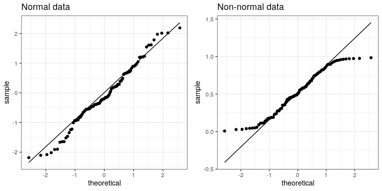

Figure 26.5: Q-Q plotsof normal (left) and non-normal (right) data. The line shows the point at which the x and y axes are equal.

Model diagnostics will be explored in more detail in the following chapter.