24.6: Appendix-

Last updated
Save as PDF

Page ID: 8846

$ \newcommand{\vecs}[1]{\overset { \scriptstyle \rightharpoonup} {\mathbf{#1}} } $ $ \newcommand{\vecd}[1]{\overset{-\!-\!\rightharpoonup}{\vphantom{a}\smash {#1}}} $$\newcommand{\id}{\mathrm{id}}$ $ \newcommand{\Span}{\mathrm{span}}$ $ \newcommand{\kernel}{\mathrm{null}\,}$ $ \newcommand{\range}{\mathrm{range}\,}$ $ \newcommand{\RealPart}{\mathrm{Re}}$ $ \newcommand{\ImaginaryPart}{\mathrm{Im}}$ $ \newcommand{\Argument}{\mathrm{Arg}}$ $ \newcommand{\norm}[1]{\| #1 \|}$ $ \newcommand{\inner}[2]{\langle #1, #2 \rangle}$ $ \newcommand{\Span}{\mathrm{span}}$ $\newcommand{\id}{\mathrm{id}}$ $ \newcommand{\Span}{\mathrm{span}}$ $ \newcommand{\kernel}{\mathrm{null}\,}$ $ \newcommand{\range}{\mathrm{range}\,}$ $ \newcommand{\RealPart}{\mathrm{Re}}$ $ \newcommand{\ImaginaryPart}{\mathrm{Im}}$ $ \newcommand{\Argument}{\mathrm{Arg}}$ $ \newcommand{\norm}[1]{\| #1 \|}$ $ \newcommand{\inner}[2]{\langle #1, #2 \rangle}$ $ \newcommand{\Span}{\mathrm{span}}$$\newcommand{\AA}{\unicode[.8,0]{x212B}}$

24.6.1 Quantifying inequality: The Gini index

Before we look at the analysis reported in the story, it’s first useful to understand how the Gini index is used to quantify inequality. The Gini index is usually defined in terms of a curve that describes the relation between income and the proportion of the population that has income at or less than that level, known as a Lorenz curve. However, another way to think of it is more intuitive: It is the relative mean absolute difference between incomes, divided by two (from https://en.Wikipedia.org/wiki/Gini_coefficient):

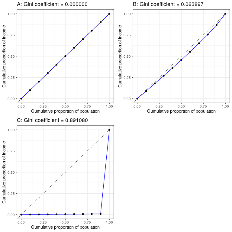
$G = \frac{\displaystyle{\sum_{i=1}^n \sum_{j=1}^n \left| x_i - x_j \right|}}{\displaystyle{2n\sum_{i=1}^n x_i}}$

Lorenz curves for A) perfect equality, B) normally distributed income, and C) high inequality (equal income except for one very wealthy individual).

Figure 24.6: Lorenz curves for A) perfect equality, B) normally distributed income, and C) high inequality (equal income except for one very wealthy individual).

Figure 24.6 shows the Lorenz curves for several different income distributions. The top left panel (A) shows an example with 10 people where everyone has exactly the same income. The length of the intervals between points are equal, indicating each person earns an identical share of the total income in the population. The top right panel (B) shows an example where income is normally distributed. The bottom left panel shows an example with high inequality; everyone has equal income ($40,000) except for one person, who has income of $40,000,000. According to the US Census, the United States had a Gini index of 0.469 in 2010, falling roughly half way between our normally distributed and maximally inequal examples.

24.6.2 Bayesian correlation analysis

We can also analyze the FiveThirtyEight data using Bayesian analysis, which has two advantages. First, it provides us with a posterior probability – in this case, the probability that the correlation value exceeds zero. Second, the Bayesian estimate combines the observed evidence with a prior, which has the effect of regularizing the correlation estimate, effectively pulling it towards zero. Here we can compute it using the jzs_cor function from the BayesMed package.

## Compiling model graph
##    Resolving undeclared variables
##    Allocating nodes
## Graph information:
##    Observed stochastic nodes: 50
##    Unobserved stochastic nodes: 4
##    Total graph size: 230
## 
## Initializing model

## $Correlation
## [1] 0.41
## 
## $BayesFactor
## [1] 11
## 
## $PosteriorProbability
## [1] 0.92

Notice that the correlation estimated using the Bayesian method is slightly smaller than the one estimated using the standard correlation coefficient, which is due to the fact that the estimate is based on a combination of the evidence and the prior, which effectively shrinks the estimate toward zero. However, notice that the Bayesian analysis is not robust to the outlier, and it still says that there is fairly strong evidence that the correlation is greater than zero.