20.8: Appendix-
- Page ID
- 8824

\( \newcommand{\vecs}[1]{\overset { \scriptstyle \rightharpoonup} {\mathbf{#1}} } \) \( \newcommand{\vecd}[1]{\overset{-\!-\!\rightharpoonup}{\vphantom{a}\smash {#1}}} \)\(\newcommand{\id}{\mathrm{id}}\) \( \newcommand{\Span}{\mathrm{span}}\) \( \newcommand{\kernel}{\mathrm{null}\,}\) \( \newcommand{\range}{\mathrm{range}\,}\) \( \newcommand{\RealPart}{\mathrm{Re}}\) \( \newcommand{\ImaginaryPart}{\mathrm{Im}}\) \( \newcommand{\Argument}{\mathrm{Arg}}\) \( \newcommand{\norm}[1]{\| #1 \|}\) \( \newcommand{\inner}[2]{\langle #1, #2 \rangle}\) \( \newcommand{\Span}{\mathrm{span}}\) \(\newcommand{\id}{\mathrm{id}}\) \( \newcommand{\Span}{\mathrm{span}}\) \( \newcommand{\kernel}{\mathrm{null}\,}\) \( \newcommand{\range}{\mathrm{range}\,}\) \( \newcommand{\RealPart}{\mathrm{Re}}\) \( \newcommand{\ImaginaryPart}{\mathrm{Im}}\) \( \newcommand{\Argument}{\mathrm{Arg}}\) \( \newcommand{\norm}[1]{\| #1 \|}\) \( \newcommand{\inner}[2]{\langle #1, #2 \rangle}\) \( \newcommand{\Span}{\mathrm{span}}\)\(\newcommand{\AA}{\unicode[.8,0]{x212B}}\)
20.8.1 Rejection sampling
We will generate samples from our posterior distribution using a simple algorithm known as rejection sampling. The idea is that we choose a random value of x (in this case
# Compute credible intervals for example
nsamples <- 100000
# create random uniform variates for x and y
x <- runif(nsamples)
y <- runif(nsamples)
# create f(x)
fx <- dbinom(x = nResponders, size = 100, prob = x)
# accept samples where y < f(x)
accept <- which(y < fx)
accepted_samples <- x[accept]
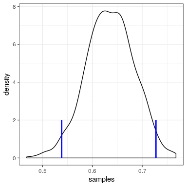
credible_interval <- quantile(x = accepted_samples,
probs = c(0.025, 0.975))
kable(credible_interval)| x | |
|---|---|
| 2.5% | 0.54 |
| 98% | 0.73 |