9.5: Z-scores

Last updated
Save as PDF

Page ID: 8763

\( \newcommand{\vecs}[1]{\overset { \scriptstyle \rightharpoonup} {\mathbf{#1}} } \) \( \newcommand{\vecd}[1]{\overset{-\!-\!\rightharpoonup}{\vphantom{a}\smash {#1}}} \)\(\newcommand{\id}{\mathrm{id}}\) \( \newcommand{\Span}{\mathrm{span}}\) \( \newcommand{\kernel}{\mathrm{null}\,}\) \( \newcommand{\range}{\mathrm{range}\,}\) \( \newcommand{\RealPart}{\mathrm{Re}}\) \( \newcommand{\ImaginaryPart}{\mathrm{Im}}\) \( \newcommand{\Argument}{\mathrm{Arg}}\) \( \newcommand{\norm}[1]{\| #1 \|}\) \( \newcommand{\inner}[2]{\langle #1, #2 \rangle}\) \( \newcommand{\Span}{\mathrm{span}}\) \(\newcommand{\id}{\mathrm{id}}\) \( \newcommand{\Span}{\mathrm{span}}\) \( \newcommand{\kernel}{\mathrm{null}\,}\) \( \newcommand{\range}{\mathrm{range}\,}\) \( \newcommand{\RealPart}{\mathrm{Re}}\) \( \newcommand{\ImaginaryPart}{\mathrm{Im}}\) \( \newcommand{\Argument}{\mathrm{Arg}}\) \( \newcommand{\norm}[1]{\| #1 \|}\) \( \newcommand{\inner}[2]{\langle #1, #2 \rangle}\) \( \newcommand{\Span}{\mathrm{span}}\)\(\newcommand{\AA}{\unicode[.8,0]{x212B}}\)

A Z-score is obtained by first subtracting the mean and then dividing by the standard deviation of a distribution. Let’s do this for the height_sample data.

mean_height <- mean(height_sample)
sd_height <- sd(height_sample)

z_height <- (height_sample - mean_height)/sd_height

Now let’s plot the histogram of Z-scores alongside the histogram for the original values. We will use the plot_grid() function from the cowplot library to plot the two figures alongside one another. First we need to put the values into a data frame, since ggplot() requires the data to be contained in a data frame.

height_df <- data.frame(orig_height=height_sample, 
                        z_height=z_height)

# create individual plots
plot_orig <- ggplot(height_df, aes(orig_height)) + 
  geom_histogram()
plot_z <- ggplot(height_df, aes(z_height)) + 
  geom_histogram()

# combine into a single figure
plot_grid(plot_orig, plot_z)

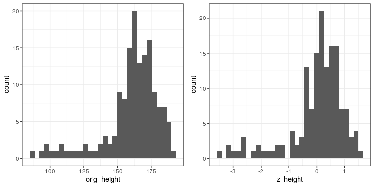
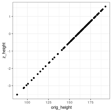
You will notice that the shapes of the histograms are similar but not exactly the same. This occurs because the binning is slightly different between the two sets of values. However, if we plot them against one another in a scatterplot, we will see that there is a direct linear relation between the two sets of values:

ggplot(height_df, aes(orig_height, z_height)) + 
  geom_point()