
5.2: Paired Data
- Page ID
- 300

Are textbooks actually cheaper online? Here we compare the price of textbooks at UCLA's bookstore and prices at Amazon.com. Seventy-three UCLA courses were randomly sampled in Spring 2010, representing less than 10% of all UCLA courses (when a class had multiple books, only the most expensive text was considered). A portion of this data set is shown in Table \(\PageIndex{1}\).
| dept | course | ucla | amazon | diff | |
|---|---|---|---|---|---|
| 1 | Am Ind | C170 | 27.67 | 27.95 | -0.28 |
| 2 | Anthro | 9 | 40.59 | 31.14 | 9.45 |
| 3 | Anthro | 135T | 31.68 | 32.00 | -0.32 |
| 4 | Anthro | 191HB | 16.00 | 11.52 | 4.48 |
| \(\vdots\) | \(\vdots\) | \(\vdots\) | \(\vdots\) | \(\vdots\) | \(\vdots\) |
| 72 | Wom Std | M144 | 23.76 | 18.72 | 5.04 |
| 73 | Wom Std | 285 | 27.70 | 18.22 | 9.48 |
Paired Observations and Samples
Each textbook has two corresponding prices in the data set: one for the UCLA bookstore and one for Amazon. Therefore, each textbook price from the UCLA bookstore has a natural correspondence with a textbook price from Amazon. When two sets of observations have this special correspondence, they are said to be paired.
Paired data
Two sets of observations are paired if each observation in one set has a special correspondence or connection with exactly one observation in the other data set.
To analyze paired data, it is often useful to look at the difference in outcomes of each pair of observations. In the textbook data set, we look at the difference in prices, which is represented as the diff variable in the textbooks data. Here the differences are taken as
\[ \text {UCLA price} - \text {Amazon price}\]
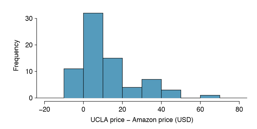
for each book. It is important that we always subtract using a consistent order; here Amazon prices are always subtracted from UCLA prices. A histogram of these differences is shown in Figure \(\PageIndex{1}\). Using differences between paired observations is a common and useful way to analyze paired data.
Exercise \(\PageIndex{1}\)
The first difference shown in Table \(\PageIndex{1}\) is computed as 27.67 - 27.95 = -0.28. Verify the differences are calculated correctly for observations 2 and 3.
Solution
- Observation 2: 40.59 - 31.14 = 9.45.
- Observation 3: 31.68 - 32.00 = -0.32.
Inference for Paired Data
To analyze a paired data set, we use the exact same tools that we developed in Chapter 4. Now we apply them to the differences in the paired observations.
| \(n_{diff}\) | \(\bar {x}_{diff}\) | \(s_{diff}\) |
|
73 |
12.76 |
14.26 |
Example \(\PageIndex{1}\): UCLA vs. Amazon
Set up and implement a hypothesis test to determine whether, on average, there is a difference between Amazon's price for a book and the UCLA bookstore's price.
Solution
There are two scenarios: there is no difference or there is some difference in average prices. The no difference scenario is always the null hypothesis:
- H0: \(\mu_{diff}\) = 0. There is no difference in the average textbook price.
- HA: \(\mu_{diff} \ne\) 0. There is a difference in average prices.
Can the normal model be used to describe the sampling distribution of \(\bar {x} _{diff}\)? We must check that the differences meet the conditions established in Chapter 4. The observations are based on a simple random sample from less than 10% of all books sold at the bookstore, so independence is reasonable; there are more than 30 differences; and the distribution of differences, shown in Figure \(\PageIndex{1}\), is strongly skewed, but this amount of skew is reasonable for this sized data set (n = 73). Because all three conditions are reasonably satisfied, we can conclude the sampling distribution of \(\bar {x}_{diff}\) nearly normal and our estimate of the standard error will be reasonable.
We compute the standard error associated with \(\bar {x} _{diff}\) using the standard deviation of the differences (\(s_{diff}\) = 14.26) and the number of differences (\(n_{diff}\) = 73):
\[ SE _{\bar {x}_{diff}} = \dfrac {s_{diff}}{\sqrt {n_{diff}}} = \dfrac {14.26}{\sqrt {73}} = 1.67\]
To visualize the p-value, the sampling distribution of \(\bar {x} _{diff}\)is drawn as though H0 is true, which is shown in Figure \(\PageIndex{1}\). The p-value is represented by the two (very) small tails.
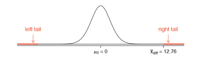
To find the tail areas, we compute the test statistic, which is the Z score of \(\bar {x} _{diff}\) under the null condition that the actual mean difference is 0:
\[ Z = \dfrac {\bar {x}_{diff} - 0}{SE _{\bar {x}_{diff}}}= \dfrac {12.76 - 0}{1.67} = 7.59\]
This Z score is so large it is not even in the table, which ensures the single tail area will be 0.0002 or smaller. Since the p-value corresponds to both tails in this case and the normal distribution is symmetric, the p-value can be estimated as twice the one-tail area:
\[ \text {p-value} = 2 \times \text {(one tail area)} \approx 2 \times 0.0002 = 0.0004\]
Because the p-value is less than 0.05, we reject the null hypothesis. We have found convincing evidence that Amazon is, on average, cheaper than the UCLA bookstore for UCLA course textbooks.
Exercise \(\PageIndex{1}\)
Create a 95% confidence interval for the average price difference between books at the UCLA bookstore and books on Amazon.
Solution
Conditions have already verified and the standard error computed in Example \(\PageIndex{1}\). To find the interval, identify \(z^*\) (1.96 for 95% confidence) and plug it, the point estimate, and the standard error into the confidence interval formula:
\[\text {point estimate} \pm z^*SE \rightarrow 12.76 \pm 1.96 \times 1.67 \rightarrow (9.49, 16.03)\]
We are 95% confident that Amazon is, on average, between $9.49 and $16.03 cheaper than the UCLA bookstore for UCLA course books.