
10.3: Two Population Means with Known Standard Deviations
- Page ID
- 779

Even though this situation is not likely (knowing the population standard deviations is not likely), the following example illustrates hypothesis testing for independent means, known population standard deviations. The sampling distribution for the difference between the means is normal and both populations must be normal. The random variable is \(\bar{X}_{1} - \bar{X}_{2}\). The normal distribution has the following format:
Normal distribution is:
\[\bar{X}_{1} - \bar{X}_{2} \sim{N}\left[\mu_{1} - \mu_{2}, \sqrt{\dfrac{(\sigma_{1})^{2}}{n_{1}} + \dfrac{(\sigma_{2})^{2}}{n_{2}}}\right] \label{eq1}\]
The standard deviation is:
\[\sqrt{\dfrac{(\sigma_{1})^{2}}{n_{1}} + \dfrac{(\sigma_{2})^{2}}{n_{2}}}\label{eq2}\]
The test statistic (z-score) is:
\[z = \dfrac{(\bar{x}_{1} - \bar{x}_{2}) - (\mu_{1} - \mu_{2})}{\sqrt{\dfrac{(\sigma_{1})^{2}}{n_{1}} + \dfrac{(\sigma_{2})^{2}}{n_{2}}}} \label{eq3}\]
Independent groups, population standard deviations known: The mean lasting time of two competing floor waxes is to be compared. Twenty floors are randomly assigned to test each wax. Both populations have a normal distributions. The data are recorded in Table.
| Wax | Sample Mean Number of Months Floor Wax Lasts | Population Standard Deviation |
|---|---|---|
| 1 | 3 | 0.33 |
| 2 | 2.9 | 0.36 |
Does the data indicate that wax 1 is more effective than wax 2? Test at a 5% level of significance.
Answer
This is a test of two independent groups, two population means, population standard deviations known.
Random Variable: \(\bar{X}_{1} - \bar{X}_{2} =\) difference in the mean number of months the competing floor waxes last.
- \(H_{0}: \mu_{1} \leq \mu_{2}\)
- \(H_{a}: \mu_{1} > \mu_{2}\)
The words "is more effective" says that wax 1 lasts longer than wax 2, on average. "Longer" is a “>” symbol and goes into \(H_{a}\). Therefore, this is a right-tailed test.
Distribution for the test: The population standard deviations are known so the distribution is normal. Using Equation \ref{eq1}, the distribution is:
\[\bar{X}_{1} - \bar{X}_{2} \sim{N} \left(0, \sqrt{\dfrac{0.33^{2}}{20} + \dfrac{0.36^{2}}{20}}\right)\]
Since \(\mu_{1} \leq \mu_{2}\) then \(\mu_{1} - \mu_{2} \leq 0\) and the mean for the normal distribution is zero.
Calculate the \(p\text{-value}\) using the normal distribution: \(p\text{-value} = 0.1799\)
Graph:
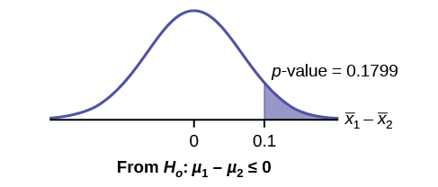
\(\bar{X}_{1} - \bar{X}_{2} = 3 – 2.9 = 0.1\)
Compare \(\alpha\) and the \(p\text{-value}\): \(\alpha = 0.05\) and \(p\text{-value} = 0.1799\). Therefore, \(\alpha < p\text{-value}\).
Make a decision: Since \(\alpha < p\text{-value}\), do not reject \(H_{0}\).
Conclusion: At the 5% level of significance, from the sample data, there is not sufficient evidence to conclude that the mean time wax 1 lasts is longer (wax 1 is more effective) than the mean time wax 2 lasts.
Press STAT. Arrow over to TESTS and press 3:2-SampZTest. Arrow over to Stats and press ENTER. Arrow down and enter .33 for sigma1, .36 for sigma2, 3 for the first sample mean, 20 for n1, 2.9 for the second sample mean, and 20 for n2. Arrow down to \(\mu1\): and arrow to \(> \mu_{2}\). Press ENTER. Arrow down to Calculate and press ENTER. The \(p\text{-value}\) is \(p = 0.1799\) and the test statistic is 0.9157. Do the procedure again, but instead of Calculatedo Dra.
The means of the number of revolutions per minute of two competing engines are to be compared. Thirty engines are randomly assigned to be tested. Both populations have normal distributions. Table shows the result. Do the data indicate that Engine 2 has higher RPM than Engine 1? Test at a 5% level of significance.
| Engine | Sample Mean Number of RPM | Population Standard Deviation |
|---|---|---|
| 1 | 1,500 | 50 |
| 2 | 1,600 | 60 |
Answer
The \(p\text{-value}\) is almost 0, so we reject the null hypothesis. There is sufficient evidence to conclude that Engine 2 runs at a higher RPM than Engine 1.
An interested citizen wanted to know if Democratic U. S. senators are older than Republican U.S. senators, on average. On May 26 2013, the mean age of 30 randomly selected Republican Senators was 61 years 247 days old (61.675 years) with a standard deviation of 10.17 years. The mean age of 30 randomly selected Democratic senators was 61 years 257 days old (61.704 years) with a standard deviation of 9.55 years.
Do the data indicate that Democratic senators are older than Republican senators, on average? Test at a 5% level of significance.
Answer
This is a test of two independent groups, two population means. The population standard deviations are unknown, but the sum of the sample sizes is 30 + 30 = 60, which is greater than 30, so we can use the normal approximation to the Student’s-t distribution. Subscripts: 1: Democratic senators 2: Republican senators
Random variable: \(\bar{X}_{1} - \bar{X}_{2} =\) difference in the mean age of Democratic and Republican U.S. senators.
- \(H_{0}: \mu_{1} \leq \mu_{2} H_{0}: \mu_{1} - \mu_{2} \leq 0\)
- \(H_{a}: \mu_{1} > \mu_{2} H_{a}: \mu_{1} - \mu_{2} > 0\)
The words "older than" translates as a “>” symbol and goes into \(H_{a}\). Therefore, this is a right-tailed test.
Distribution for the test: The distribution is the normal approximation to the Student’s t for means, independent groups. Using the formula, the distribution is: \[\bar{X}_{1} - \bar{X}_{2} \sim N\left[0, \sqrt{\dfrac{(9.55)^{2}}{30} + \dfrac{(10.17)^{2}}{30}}\right]\]
Since \(\mu_{1} \leq \mu_{2}, \mu_{1} - \mu_{2} \leq 0\) and the mean for the normal distribution is zero.
(Calculating the p-value using the normal distribution gives \(p\text{-value} = 0.4040\))
Graph:
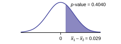
Compare \(\alpha\) and the \(p\text{-value}\): \(\alpha = 0.05\) and \(p\text{-value} = 0.4040\). Therefore, \(\alpha < p\text{-value}\).
Make a decision: Since \(\alpha < p\text{-value}\), do not reject \(H_{0}\).
Conclusion: At the 5% level of significance, from the sample data, there is not sufficient evidence to conclude that the mean age of Democratic senators is greater than the mean age of the Republican senators.
References
- Data from the United States Census Bureau. Available online at www.census.gov/prod/cen2010/b...c2010br-02.pdf
- Hinduja, Sameer. “Sexting Research and Gender Differences.” Cyberbulling Research Center, 2013. Available online at cyberbullying.us/blog/sexting...r-differences/ (accessed June 17, 2013).
- “Smart Phone Users, By the Numbers.” Visually, 2013. Available online at http://visual.ly/smart-phone-users-numbers (accessed June 17, 2013).
- Smith, Aaron. “35% of American adults own a Smartphone.” Pew Internet, 2013. Available online at www.pewinternet.org/~/media/F...martphones.pdf (accessed June 17, 2013).
- “State-Specific Prevalence of Obesity AmongAduls—Unites States, 2007.” MMWR, CDC. Available online at http://www.cdc.gov/mmwr/preview/mmwrhtml/mm5728a1.htm (accessed June 17, 2013).
- “Texas Crime Rates 1960–1012.” FBI, Uniform Crime Reports, 2013. Available online at: http://www.disastercenter.com/crime/txcrime.htm (accessed June 17, 2013).
Review
A hypothesis test of two population means from independent samples where the population standard deviations are known will have these characteristics:
- Random variable: \(\overline{X}_1−\overline{X}_2 =\) the difference of the means
- Distribution: normal distribution
Formula Review
Normal Distribution:
\[\bar{X}_{1} - \bar{X}_{2} = \sim N\left[\mu_{1} - \mu_{2}, \sqrt{\dfrac{(\sigma_{1})^{2}}{n_{1}} + \dfrac{(\sigma_{2})^{2}}{n_{2}}}\right]\]
Generally \(\mu_{1} - \mu_{2} = 0\).
Test Statistic (z-score):
\[z = \dfrac{(\bar{x}_{1} - \bar{x}_{2}) - (\mu_{1} - \mu_{2})}{\sqrt{\dfrac{(\sigma_{1})^{2}}{n_{1}} + \dfrac{(\sigma_{2})^{2}}{n_{2}}}}\]
Generally \(\mu_{1} - \mu_{2} = 0\).
where:
\(\sigma_{1}\) and \(\sigma_{2}\) are the known population standard deviations. \(n_{1}\) and \(n_{1}\) are the sample sizes. \(\bar{x}_{1}\) and \(\bar{x}_{2}\) are the sample means. \(\mu_{1}\) and \(\mu_{2}\) are the population means