9.6: Difference Between Means

Last updated
Save as PDF

Page ID: 2136

\( \newcommand{\vecs}[1]{\overset { \scriptstyle \rightharpoonup} {\mathbf{#1}} } \) \( \newcommand{\vecd}[1]{\overset{-\!-\!\rightharpoonup}{\vphantom{a}\smash {#1}}} \)\(\newcommand{\id}{\mathrm{id}}\) \( \newcommand{\Span}{\mathrm{span}}\) \( \newcommand{\kernel}{\mathrm{null}\,}\) \( \newcommand{\range}{\mathrm{range}\,}\) \( \newcommand{\RealPart}{\mathrm{Re}}\) \( \newcommand{\ImaginaryPart}{\mathrm{Im}}\) \( \newcommand{\Argument}{\mathrm{Arg}}\) \( \newcommand{\norm}[1]{\| #1 \|}\) \( \newcommand{\inner}[2]{\langle #1, #2 \rangle}\) \( \newcommand{\Span}{\mathrm{span}}\) \(\newcommand{\id}{\mathrm{id}}\) \( \newcommand{\Span}{\mathrm{span}}\) \( \newcommand{\kernel}{\mathrm{null}\,}\) \( \newcommand{\range}{\mathrm{range}\,}\) \( \newcommand{\RealPart}{\mathrm{Re}}\) \( \newcommand{\ImaginaryPart}{\mathrm{Im}}\) \( \newcommand{\Argument}{\mathrm{Arg}}\) \( \newcommand{\norm}[1]{\| #1 \|}\) \( \newcommand{\inner}[2]{\langle #1, #2 \rangle}\) \( \newcommand{\Span}{\mathrm{span}}\)\(\newcommand{\AA}{\unicode[.8,0]{x212B}}\)

Learning Objectives

State the mean and variance of the sampling distribution of the difference between means
Compute the standard error of the difference between means
Compute the probability of a difference between means being above a specified value

Statistical analyses are very often concerned with the difference between means. A typical example is an experiment designed to compare the mean of a control group with the mean of an experimental group. Inferential statistics used in the analysis of this type of experiment depend on the sampling distribution of the difference between means.

The sampling distribution of the difference between means can be thought of as the distribution that would result if we repeated the following three steps over and over again:

sample \(n_1\) scores from \(\text {Population 1}\) and \(n_2\) scores from \(\text {Population 2}\)
compute the means of the two samples (\(M_1\)and \(M_2\))
compute the difference between means, \(M_1-M_2\)

The distribution of the differences between means is the sampling distribution of the difference between means.

As you might expect, the mean of the sampling distribution of the difference between means is:

\[\mu _{M_1-M_2}=\mu _1-\mu _2\]

which says that the mean of the distribution of differences between sample means is equal to the difference between population means. For example, say that the mean test score of all \(12\)-year-olds in a population is \(34\) and the mean of \(10\)-year-olds is \(25\). If numerous samples were taken from each age group and the mean difference computed each time, the mean of these numerous differences between sample means would be \(34-25=9\).

From the variance sum law, we know that:

\[\sigma _{M_1-M_2}^{2}=\sigma _{M_1}^{2}+\sigma _{M_2}^{2}\]

which says that the variance of the sampling distribution of the difference between means is equal to the variance of the sampling distribution of the mean for \(\text {Population 1}\) plus the variance of the sampling distribution of the mean for \(\text {Population 2}\). Recall the formula for the variance of the sampling distribution of the mean:

\[\sigma _{M}^{2}=\frac{\sigma ^2}{N}\]

Since we have two populations and two samples sizes, we need to distinguish between the two variances and sample sizes. We do this by using the subscripts \(1\) and \(2\). Using this convention, we can write the formula for the variance of the sampling distribution of the difference between means as:

\[\sigma _{M_1-M_2}^{2}=\frac{\sigma _1^2}{n_1}+\frac{\sigma _2^2}{n_2}\]

Since the standard error of a sampling distribution is the standard deviation of the sampling distribution, the standard error of the difference between means is:

\[\sigma _{M_1-M_2}=\sqrt{\frac{\sigma _1^2}{n_1}+\frac{\sigma _2^2}{n_2}}\]

Just to review the notation, the symbol on the left contains a sigma (\(\sigma\)), which means it is a standard deviation. The subscripts \(M_1-M_2\) indicate that it is the standard deviation of the sampling distribution of \(M_1-M_2\).

Now let's look at an application of this formula.

Example \(\PageIndex{1}\)

Assume there are two species of green beings on Mars. The mean height of \(\text{Species 1}\) is \(32\) while the mean height of \(\text{Species 2}\) is \(22\). The variances of the two species are \(60\) and \(70\), respectively and the heights of both species are normally distributed. You randomly sample \(10\) members of \(\text{Species 1}\) and \(14\) members of \(\text{Species 2}\). What is the probability that the mean of the \(10\) members of \(\text{Species 1}\) will exceed the mean of the \(14\) members of \(\text{Species 2}\) by \(5\) or more? Without doing any calculations, you probably know that the probability is pretty high since the difference in population means is \(10\). But what exactly is the probability?

Solution

First, let's determine the sampling distribution of the difference between means. Using the formulas above, the mean is

\[\mu _{M_1-M_2}=32-22=10\]

The standard error is:

\[\sigma _{M_1-M_2}=\sqrt{\frac{60}{10}+\frac{70}{14}}=3.317\]

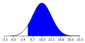
The sampling distribution is shown in Figure \(\PageIndex{1}\). Notice that it is normally distributed with a mean of \(10\) and a standard deviation of \(3.317\). The area above \(5\) is shaded blue.

sampling distribution.gif — Figure \(\PageIndex{1}\): The sampling distribution of the difference between means

The last step is to determine the area that is shaded blue. Using either a \(Z\) table or the normal calculator, the area can be determined to be \(0.934\). Thus the probability that the mean of the sample from \(\text{Species 1}\) will exceed the mean of the sample from \(\text{Species 2}\) by \(5\) or more is \(0.934\).

As shown below, the formula for the standard error of the difference between means is much simpler if the sample sizes and the population variances are equal. When the variances and samples sizes are the same, there is no need to use the subscripts \(1\) and \(2\) to differentiate these terms.

\[\sigma _{M_1-M_2}=\sqrt{\frac{\sigma _1^2}{n_1}+\frac{\sigma _2^2}{n_2}}=\sqrt{\frac{\sigma ^2}{n}+\frac{\sigma ^2}{n}}=\sqrt{\frac{2\sigma ^2}{n}}\]

This simplified version of the formula can be used for the following problem.

Example \(\PageIndex{2}\)

The mean height of \(15\)-year-old boys (in cm) is \(175\) and the variance is \(64\). For girls, the mean is \(165\) and the variance is \(64\). If eight boys and eight girls were sampled, what is the probability that the mean height of the sample of girls would be higher than the mean height of the sample of boys? In other words, what is the probability that the mean height of girls minus the mean height of boys is greater than \(0\)?

Solution

As before, the problem can be solved in terms of the sampling distribution of the difference between means (girls - boys). The mean of the distribution is 165 - 175 = -10. The standard deviation of the distribution is:

\[\sigma _{M_1-M_2}=\sqrt{\frac{2\sigma ^2}{n}}=\sqrt{\frac{(2)(64)}{8}}=4\]

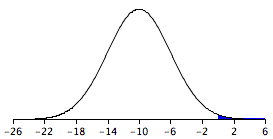
A graph of the distribution is shown in Figure \(\PageIndex{2}\). It is clear that it is unlikely that the mean height for girls would be higher than the mean height for boys since in the population boys are quite a bit taller. Nonetheless it is not inconceivable that the girls' mean could be higher than the boys' mean.

boy_girl example.gif — Figure \(\PageIndex{2}\): Sampling distribution of the difference between mean heights

A difference between means of 0 or higher is a difference of \(10/4 = 2.5\) standard deviations above the mean of \(-10\). The probability of a score \(2.5\) or more standard deviations above the mean is \(0.0062\).