5.3: Predicting Across Data Sets

As we saw in the previous section, data splitting is a useful technique for testing a regression model. If you have other data sets, you can use them to further test your new model’s capabilities.

In our situation, we have several additional benchmark results in the data file that we can use for these tests. As an example, we use the model we developed from the Int2000 data to predict the Fp2000 benchmark’s performance.

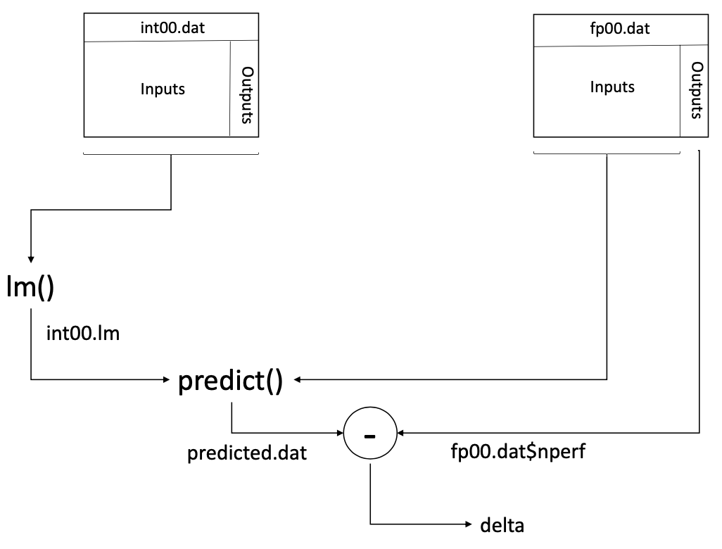
We first train the model developed using the Int2000 data, int00.lm, using all the Int2000 data available in the int00.dat data frame. We then predict the Fp2000 results using this model and the fp00.dat data. Again, we assign the differences between the predicted and actual results to the vector delta. Figure 5.3 shows the overall data flow for this training and testing. The corresponding R commands are:

> int00.lm <lm(nperf ~ clock + cores + voltage + channel + 
L1icache + sqrt(L1icache) + L1dcache + sqrt(L1dcache) + L2cache + 
sqrt(L2cache), data = int00.dat)> predicted.dat <predict(int00.lm, newdata=fp00.dat) 
> delta <predicted.dat fp00.dat$nperf
> t.test(delta, conf.level = 0.95)

One Sample t-test

data: delta
t = 1.5231, df = 80, p-value = 0.1317
alternative hypothesis: true mean is not equal to 0 
95 percent confidence interval:
-0.4532477 3.4099288 sample estimates:
mean of x
1.478341

 

Figure 5.3: Predicting the Fp2000 results using the model developed with the Int2000 data.

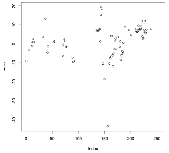
The resulting confidence interval for the delta values contains zero and is relatively small. This result suggests that the model developed using the Int2000 data is reasonably good at predicting the Fp2000 benchmark program’s results. The scatter plot in Figure 5.4 shows the resulting delta values for each of the processors we used in the prediction. The results tend to be randomly distributed around zero, as we would expect from a good regression model. Note, however, that some of the values differ significantly from zero. The maximum positive deviation is almost 20, and the magnitude of the largest negative value is greater than 43. The confidence interval suggests relatively good results, but this scatter plot shows that not all the values are well predicted.

Figure 5.4: A scatter plot of the differences between the predicted and actual performance results for the Fp2000 benchmark when predicted using the Int2000 regression model.

As a final example, we use the Int2000 regression model to predict the results of the benchmark program’s future Int2006 version. The R code to compute this prediction is:

> int00.lm <lm(nperf ~ clock + cores + voltage + channel + L1icache + sqrt(L1icache) + L1dcache + 
sqrt(L1dcache) + L2cache + sqrt(L2cache), data = int00.dat)> predicted.dat <predict(int00.lm, newdata=int06.dat) 
> delta <predicted.dat int06.dat$nperf
> t.test(delta, conf.level = 0.95)

One Sample t-test

data: delta
t = 49.339, df = 168, p-value < 2.2e-16
alternative hypothesis: true mean is not equal to 0 
95 percent confidence interval: 48.87259 52.94662
sample estimates: 
mean of x
  50.9096

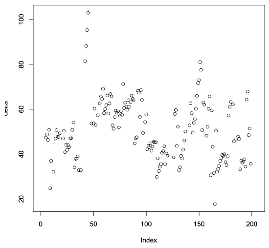
In this case, the confidence interval for the delta values does not include zero. In fact, the mean value of the differences is 50.9096, which indicates that the average of the model-predicted values is substantially larger than the actual average value. The scatter plot shown in Figure 5.5 further confirms that the predicted values are all much larger than the actual values. 

This example is a good reminder that models have their limits. Apparently, there are more factors that affect the performance of the next generation of the benchmark programs, Int2006, than the model we developed using the Int2000 results captures. To develop a model that better predicts future performance, we would have to uncover those factors. Doing so requires a deeper understanding of the factors that affect computer performance, which is beyond the scope of this tutorial.

Figure 5.5: A scatter plot of the differences between the predicted and actual performance results for the Int2006 benchmark, predicted using the Int2000 regression model.