4.2: Identifying Potential Predictors

The first step in developing the multi-factor regression model is to identify all possible predictors that we could include in the model. To the novice model developer, it may seem that we should include all factors available in the data as predictors, because more information is likely to be better than not enough information. However, a good regression model explains the relationship between a system’s inputs and output as simply as possible. Thus, we should use the smallest number of predictors necessary to provide good predictions. Furthermore, using too many or redundant predictors builds the random noise in the data into the model. In this situation, we obtain an over-fitted model that is very good at predicting the outputs from the specific input data set used to train the model. It does not accurately model the overall system’s response, though, and it will not appropriately predict the system output for a broader range of inputs than those on which it was trained. Redundant or unnecessary predictors also can lead to numerical instabilities when computing the coefficients.

We must find a balance between including too few and too many predictors. A model with too few predictors can produce biased predictions. On the other hand, adding more predictors to the model will always cause the R² value to increase. This can confuse you into thinking that the additional predictors generated a better model. In some cases, adding a predictor will improve the model, so the increase in the R² value makes sense. In some cases, however, the R² value increases simply because we’ve better modeled the random noise.

The adjusted R² attempts to compensate for the regular R²’s behavior by changing the R² value according to the number of predictors in the model. This adjustment helps us determine whether adding a predictor improves the fit of the model, or whether it is simply modeling the noise better. It is computed as:

\(\ R_{adjusted}^2 = {1-\frac{n-1}{n-m}(1-R^2)}\)

where n is the number of observations and m is the number of predictors in the model. If adding a new predictor to the model increases the previous model’s R² value by more than we would expect from random fluctuations, then the adjusted R² will increase. Conversely, it will decrease if removing a predictor decreases the R² by more than we would expect due to random variations. Recall that the goal is to use as few predictors as possible, while still producing a model that explains the data well.

Because we do not know a priori which input parameters will be useful predictors, it seems reasonable to start with all of the columns available in the measured data as the set of potential predictors. We listed all of the column names in Table 2.1. Before we throw all these columns into the modeling process, though, we need to step back and consider what we know about the underlying system, to help us find any parameters that we should obviously exclude from the start.

There are two output columns: perf and nperf. The regression model can have only one output, however, so we must choose only one column to use in our model development process. As discussed in Section 4.1, nperf is a linear transformation of perf that shifts the output range to be between 0 and 100. This range is useful for quickly obtaining a sense of future predictions’ quality, so we decide to use nperf as our model’s output and ignore the perf column.

Almost all the remaining possible predictors appear potentially useful in our model, so we keep them available as potential predictors for now. The only exception is TDP. The name of this factor, thermal design power, does not clearly indicate whether this could be a useful predictor in our model, so we must do a little additional research to understand it better. We discover [10] that thermal design power is “the average amount of power in watts that a cooling system must dissipate. Also called the ‘thermal guideline’ or ‘thermal design point,’ the TDP is provided by the chip manufacturer to the system vendor, who is expected to build a case that accommodates the chip’s thermal requirements.” From this definition, we conclude that TDP is not really a parameter that will directly affect performance. Rather, it is a specification provided by the processor’s manufacturer to ensure that the system designer includes adequate cooling capability in the final product. Thus, we decide not to include TDP as a potential predictor in the regression model.

In addition to excluding some apparently unhelpful factors (such as TDP) at the beginning of the model development process, we also should consider whether we should include any additional parameters. For example, the terms in a regression model add linearly to produce the predicted output. However, the individual terms themselves can be nonlinear, such as aixim ,where m does not have to be equal to one.This flexibility lets us include additional powers of the individual factors. We should include these non-linear terms, though, only if we have some physical reason to suspect that the output could be a nonlinear function of a particular input.

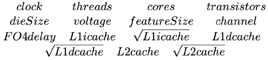
For example, we know from our prior experience modeling processor performance that empirical studies have suggested that cache miss rates are roughly proportional to the square root of the cache size [5]. Consequently, we will include terms for the square root (m = 1/2) of each cache size as possible predictors. We must also include first-degree terms (m = 1) of each cache size as possible predictors. Finally, we notice that only a few of the entries in the int00.dat data frame include values for the L3 cache, so we decide to exclude the L3 cache size as a potential predictor. Exploiting this type of domain-specific knowledge when selecting predictors ultimately can help produce better models than blindly applying the model development process.

The final list of potential predictors that we will make available for the model development process is shown in Table 4.1.

Table 4.1: The list of potential predictors to be used in the model development process.