14.2: Interaction Effects

Dummy variables can also be used to estimate the ways in which the effect of a variable differs across subsets of cases. These kinds of effects are generally called interactions." When an interaction occurs, the effect of one XX is dependent on the value of another. Typically, an OLS model is additive, where the BB’s are added together to predict YY;

Yi=A+BX1+BX2+BX3+BX4+EiYi=A+BX1+BX2+BX3+BX4+Ei.

However, an interaction model has a multiplicative effect where two of the IVs are multiplied;

Yi=A+BX1+BX2+BX3∗BX4+EiYi=A+BX1+BX2+BX3∗BX4+Ei.

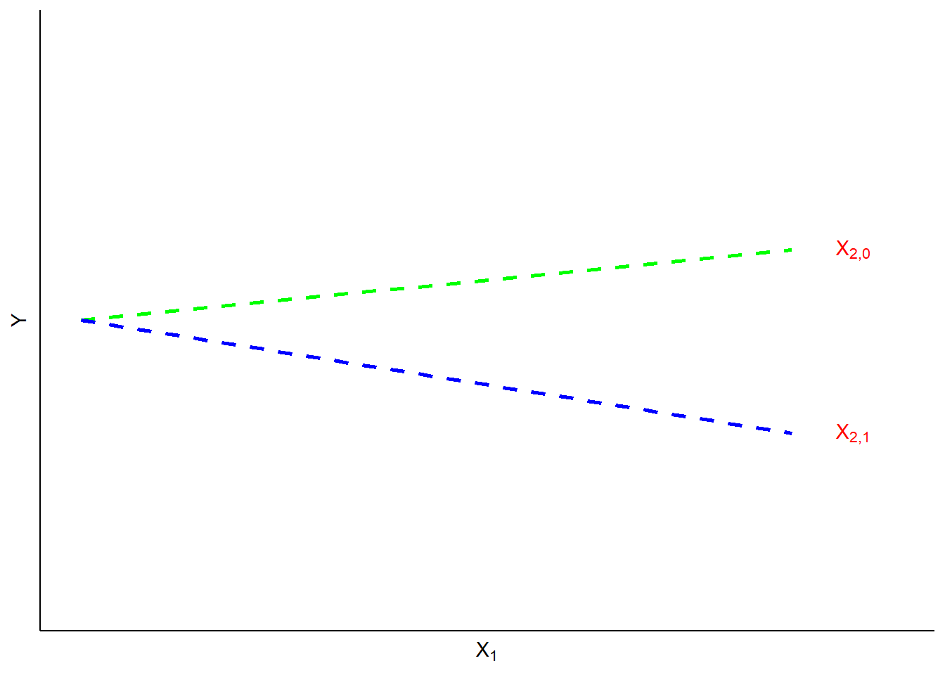
A slope dummy" is a special kind of interaction in which a dummy variable is interacted with (multiplied by) a scale (ordinal or higher) variable. Suppose, for example, that you hypothesized that the effects of political of ideology on perceived risks of climate change were different for men and women. Perhaps men are more likely than women to consistently integrate ideology into climate change risk perceptions. In such a case, a dummy variable (0=women, 1=men) could be interacted with ideology (1=strong liberal, 7=strong conservative) to predict levels of perceived risk of climate change (0=no risk, 10=extreme risk). If your hypothesized interaction was correct, you would observe the kind of pattern as shown in Figure \(\PageIndex{2}\).

Figure \(\PageIndex{2}\): Illustration of Slope Interaction

We can test our hypothesized interaction in R, controlling for the effects of age and income.

ols2 <- lm(glbcc_risk ~ age + income + education + gender * ideol, data = ds.temp)
summary(ols2)

## 
## Call:
## lm(formula = glbcc_risk ~ age + income + education + gender * 
##     ideol, data = ds.temp)
## 
## Residuals:
##    Min     1Q Median     3Q    Max 
## -8.718 -1.704  0.166  1.468  6.929 
## 
## Coefficients:
##                   Estimate    Std. Error t value             Pr(>|t|)    
## (Intercept)  10.6004885194  0.3296900513  32.153 < 0.0000000000000002 ***
## age          -0.0041366805  0.0036653120  -1.129              0.25919    
## income       -0.0000023222  0.0000009069  -2.561              0.01051 *  
## education     0.0682885587  0.0299249903   2.282              0.02258 *  
## gender        0.5971981026  0.2987398877   1.999              0.04572 *  
## ideol        -0.9591306050  0.0389448341 -24.628 < 0.0000000000000002 ***
## gender:ideol -0.1750006234  0.0597401590  -2.929              0.00343 ** 
## ---
## Signif. codes:  0 '***' 0.001 '**' 0.01 '*' 0.05 '.' 0.1 ' ' 1
## 
## Residual standard error: 2.427 on 2264 degrees of freedom
## Multiple R-squared:  0.3664, Adjusted R-squared:  0.3647 
## F-statistic: 218.2 on 6 and 2264 DF,  p-value: < 0.00000000000000022

The results indicate a negative and significant interaction effect for gender and ideology. Consistent with our hypothesis, this means that the effect of ideology on climate change risk is more pronounced for males than females. Put differently, the slope of ideology is steeper for males than it is for females. This is shown in Figure \(\PageIndex{3}\).

ds.temp$gend.factor <- factor(ds.temp$gender, levels=c(0,1),labels=c("Female","Male"))
library(effects)
ols3 <- lm(glbcc_risk~ age + income + education + ideol * gend.factor, data = ds.temp)
plot(effect("ideol*gend.factor",ols3),ylim=0:10)

Figure \(\PageIndex{3}\): Interaction of Ideology and Gender

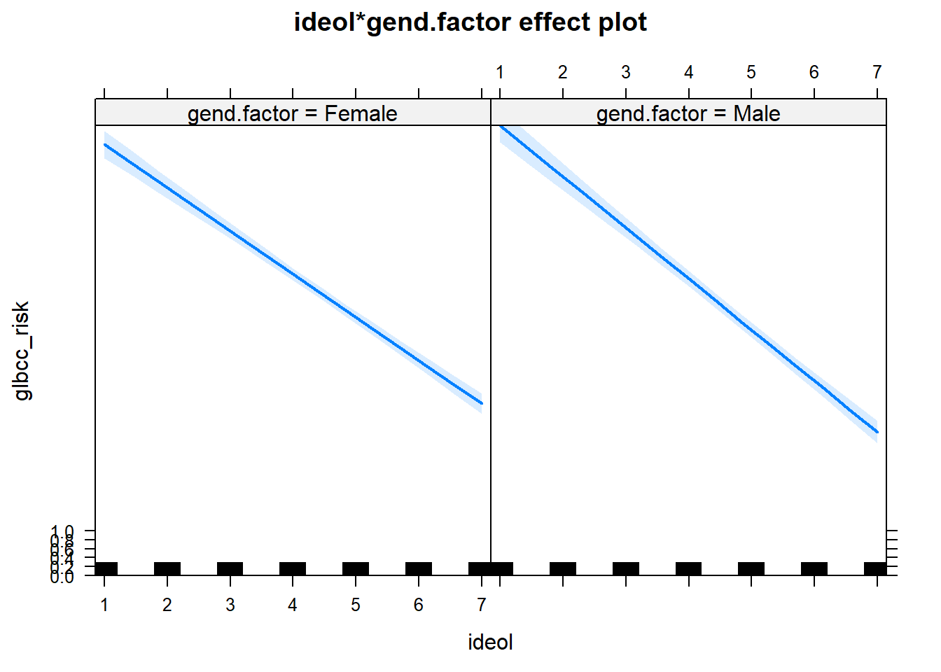
In sum, dummy variables add greatly to the flexibility of OLS model specification. They permit the inclusion of categorical variables, and they allow for testing hypotheses about interactions of groups with other IVs within the model. This kind of flexibility is one reason that OLS models are widely used by social scientists and policy analysts.