10.3: Application of Residual Diagnostics
- Page ID
- 7249
This far we have used rather simple illustrations of residual diagnostics and the kinds of patterns to look for. But you should be warned that, in real applications, the patterns are rarely so clear. So we will walk through an example diagnostic session, using the the tbur data set.
Our in-class lab example focuses on the relationship between political ideology (“ideology” in our dataset) as a predictor of the perceived risks posed by climate change (“gccrsk”). The model is specified in R as follows:
OLS_env <- lm(ds$glbcc_risk ~ ds$ideol)Using the summary command in R, we can review the results.
summary(OLS_env)##
## Call:
## lm(formula = ds$glbcc_risk ~ ds$ideol)
##
## Residuals:
## Min 1Q Median 3Q Max
## -8.726 -1.633 0.274 1.459 6.506
##
## Coefficients:
## Estimate Std. Error t value Pr(>|t|)
## (Intercept) 10.81866 0.14189 76.25 <0.0000000000000002 ***
## ds$ideol -1.04635 0.02856 -36.63 <0.0000000000000002 ***
## ---
## Signif. codes: 0 '***' 0.001 '**' 0.01 '*' 0.05 '.' 0.1 ' ' 1
##
## Residual standard error: 2.479 on 2511 degrees of freedom
## (34 observations deleted due to missingness)
## Multiple R-squared: 0.3483, Adjusted R-squared: 0.348
## F-statistic: 1342 on 1 and 2511 DF, p-value: < 0.00000000000000022Note that, as was discussed in the prior chapter, the estimated value for BB is negative and highly statistically significant. This indicates that the more conservative the survey respondent, the lower the perceived risks attributed to climate change. Now we will use these model results and the associated residuals to evaluate the key assumptions of OLS, beginning with linearity.
10.3.1 Testing for Non-Linearity
One way to test for non-linearity is to fit the model to a polynomial functional form. This sounds impressive but is quite easy to do and understand (really!). All you need to do is include the square of the independent variable as a second predictor in the model. A significant regression coefficient on the squared variable indicates problems with linearity. To do this, we first produce the squared variable.
#first we square the ideology variable and create a new variable to use in our model.
ds$ideology2 <- ds$ideol^2
summary(ds$ideology2)
## Min. 1st Qu. Median Mean 3rd Qu. Max. NA's
## 1.00 16.00 25.00 24.65 36.00 49.00 23Next, we run the regression with the original independent variable and our new squared variable. Finally, we check the regression output.
OLS_env2 <- lm(glbcc_risk ~ ideol + ideology2, data = ds)
summary(OLS_env2)
A significant coefficient on the squared ideology variable informs us that we probably have a non-linearity problem. The significant and negative coefficient for the square of ideology means that the curve steepens (perceived risks fall faster) as the scale shifts further up on the conservative side of the scale. We can supplement the polynomial regression test by producing a residual plot with a formal Tukey test. The residual plot (car package residualPlots function) displays the Pearson fitted values against the model’s observed values. Ideally, the plots will produce flat red lines; curved lines represent non-linearity. The output for the Tukey test is visible in the RR workspace. The null hypothesis for the Tukey test is a linear relationship, so a significant p-value is indicative of non-linearity. The tukey test is reported as part of the residualPlots function in the car package.
#A significant p-value indicates non-linearity using the Tukey test
library(car)
residualPlots(OLS_env)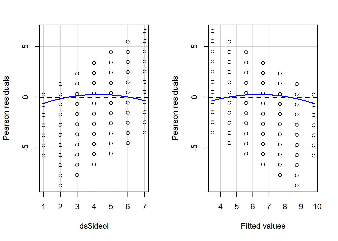
##            Test stat Pr(>|Test stat|)
## ds$ideol     -5.0181     0.0000005584 ***
## Tukey test   -5.0181     0.0000005219 ***
## ---
## Signif. codes:  0 '***' 0.001 '**' 0.01 '*' 0.05 '.' 0.1 ' ' 1
The curved red lines in Figure \(\PageIndex{7}\) in the residual plots and significant Tukey test indicate a non-linear relationship in the model. This is a serious violation of a core assumption of OLS regression, which means that the estimate of BB is likely to be biased. Our findings suggest that the relationship between ideology and perceived risks of climate change is approximately linear from “strong liberals” to those who are “leaning Republican”. But perceived risks seem to drop off more rapidly as the scale rises toward “strong Republican.”
10.3.2 Testing for Normality in Model Residuals
Testing for normality in the model residuals will involve using many of the techniques demonstrated in previous chapters. The first step is to graphically display the residuals in order to see how closely the model residuals resemble a normal distribution. A formal test for normality is also included in the demonstration.
Start by creating a histogram of the model residuals.
OLS_env$residuals %>% # Pipe the residuals to a data frame
  data.frame() %>% # Pipe the data frame to ggplot
  ggplot(aes(OLS_env$residuals)) +
  geom_histogram(bins = 16)
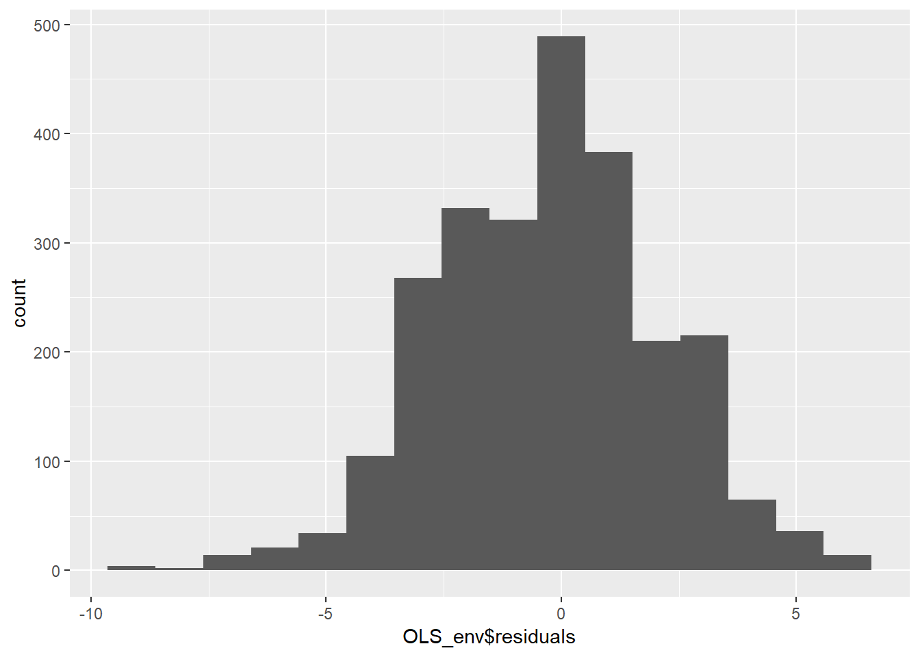
The histogram in figure 10.8 indicates that the residuals are approximately normally distributed, but there appears to be a negative skew. Next, we can create a smoothed density of the model residuals compared to a theoretical normal distribution.
OLS_env$residuals %>% # Pipe the residuals to a data frame
  data.frame() %>% # Pipe the data frame to ggplot
  ggplot(aes(OLS_env$residuals)) +
  geom_density(adjust = 2) +
  stat_function(fun = dnorm, args = list(mean = mean(OLS_env$residuals),
                                         sd = sd(OLS_env$residuals)),
                color = "red")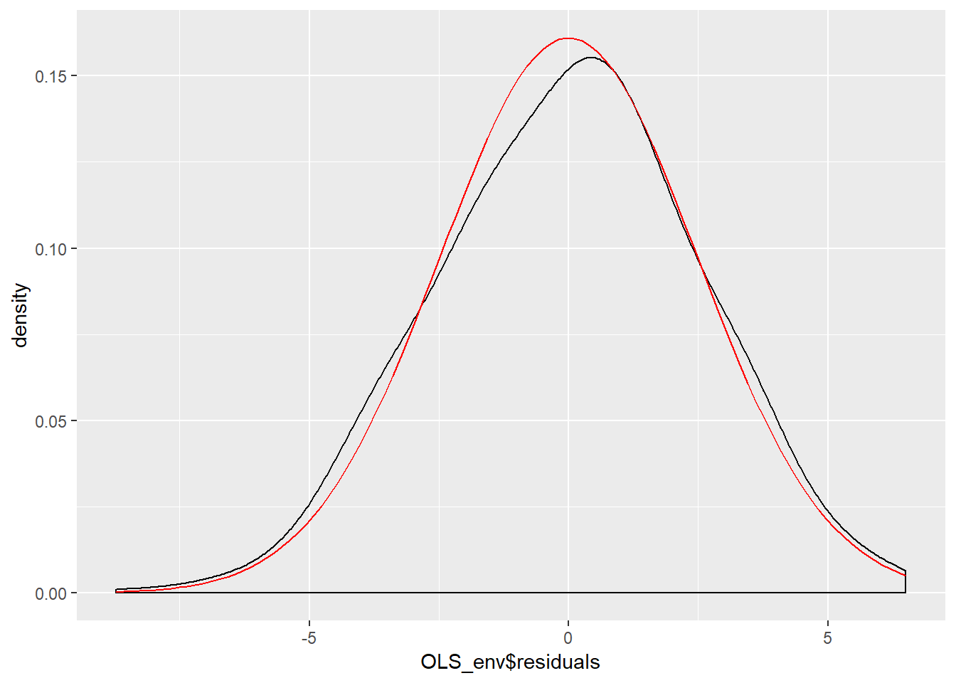
Figure \(\PageIndex{9}\) indicates the model residuals deviate slightly from a normal distributed because of a slightly negative skew and a mean higher than we would expect in a normal distribution. Our final ocular examination of the residuals will be a quartile plot %(using the stat_qq function from the ggplot2 package).
OLS_env$residuals %>% # Pipe the residuals to a data frame
  data.frame() %>% # Pipe the data frame to ggplot
  ggplot(aes(sample = OLS_env$residuals)) +
  stat_qq() +
  stat_qq_line()
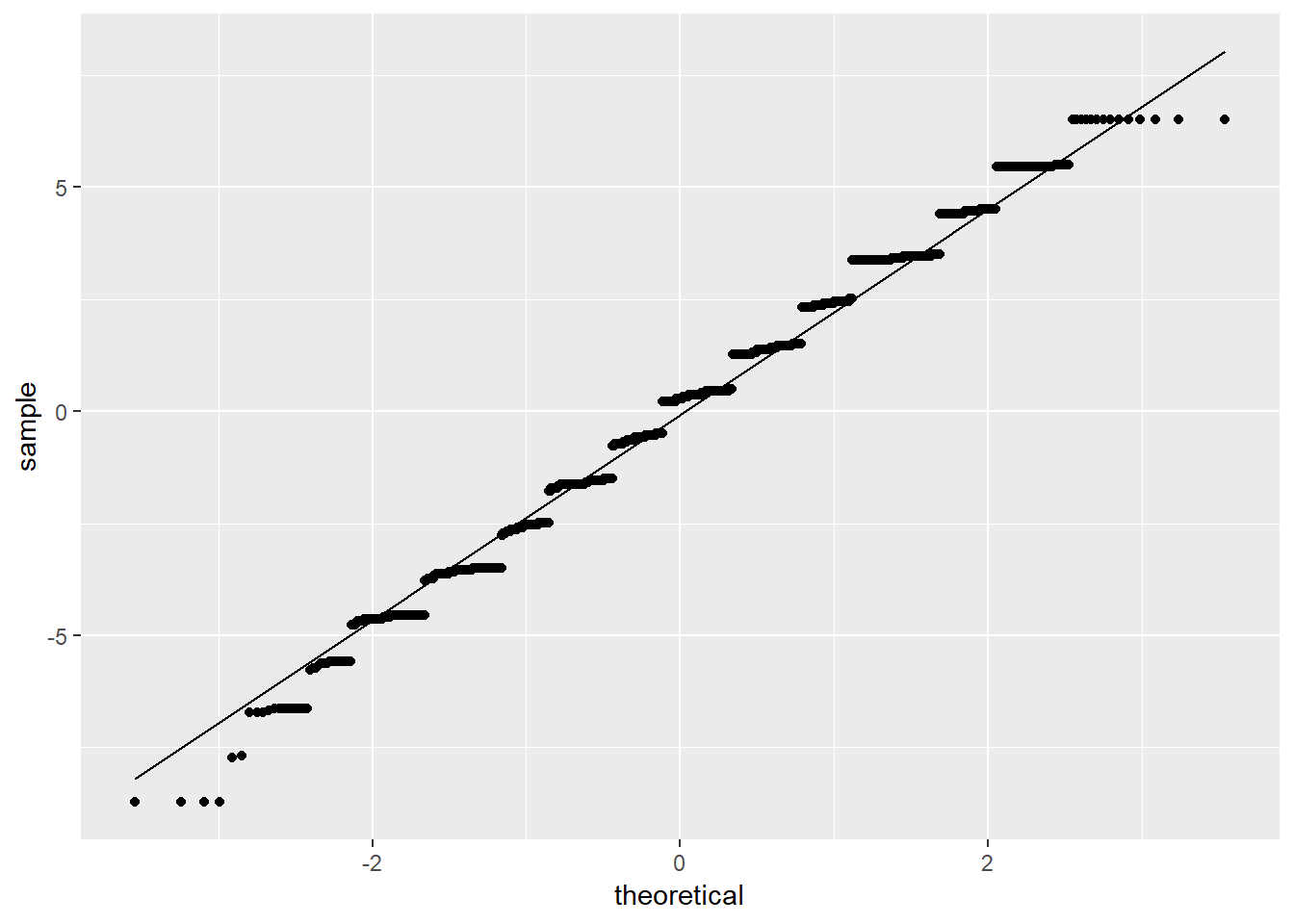
According to Figure \(\PageIndex{10}\), it appears as if the residuals are normally distributed except for the tails of the distribution. Taken together the graphical representations of the residuals suggest modest non-normality. As a final step, we can conduct a formal Shapiro-Wilk test for normality. The null hypothesis for a Shapiro-Wilk test is a normal distribution, so we do not want to see a significant p-value.
#a significant value p-value potentially indicates the data is not normally distributed.
shapiro.test(OLS_env$residuals)
##
## Shapiro-Wilk normality test
##
## data: OLS_env$residuals
## W = 0.98901, p-value = 0.000000000000551The Shapiro-Wilk test confirms what we observed in the graphical displays of the model residuals – the residuals are not normally distributed. Recall that our dependent variable (gccrsk) appears to have a non-normal distribution. This could be the root of the non-normality found in the model residuals. Given this information, steps must be taken to assure that the model residuals meet the required OLS assumptions. One possibility would be to transform the dependent variable (glbccrisk) in order to induce a normal distribution. Another might be to add a polynomial term to the independent variable (ideology) as was done above. In either case, you would need to recheck the residuals in order to see if the model revisions adequately dealt with the problem. We suggest that you do just that!
10.3.3 Testing for Non-Constant Variance in the Residuals
Testing for non-constant variance (heteroscedasticity) in a model is fairly straightforward. We can start by creating a spread-level plot that fits the studentized residuals against the model’s fitted values. A line with a non-zero slope is indicative of heteroscedasticity. Figure \(\PageIndex{11}\) displays the spread-level plot from the car package.
spreadLevelPlot(OLS_env)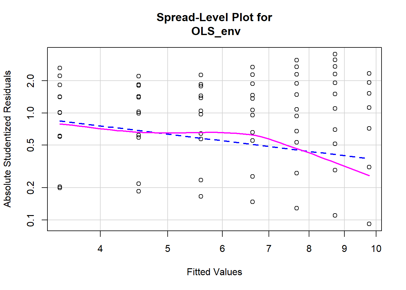
##
## Suggested power transformation: 1.787088dev.off() ## RStudioGD
## 2The negative slope on the red line in Figure \(\PageIndex{11}\) indicates the model may contain heteroscedasticity. We can also perform a formal test for non constant variance. The null hypothesis is constant variance, so we do not want to see a significant p-value.
#a significant value indicates potential heteroscedasticity issues.
ncvTest(OLS_env)
## Non-constant Variance Score Test
## Variance formula: ~ fitted.values
## Chisquare = 68.107 Df = 1 p = 0.0000000000000001548597The significant p-value on the non-constant variance test informs us that there is a problem with heteroscedasticity in the model. This is yet another violation of the core assumptions of OLS regression, and it brings into doubt our hypothesis tests.
10.3.4 Examining Outlier Data
There are a number of ways to examine outlying observations in an OLS regression. This section briefly illustrates a subset of analytical tests that will provide a useful assessment of potentially important outliers. The purpose of examining outlier data is twofold. First, we want to make sure there are not any mis-coded or invalid data influencing our regression. For example, an outlying observation with a value of “-99” would very likely bias our results and obviously needs to be corrected. Second, outlier data may indicate the need to theoretically reconceptualize our model. Perhaps the relationship in the model is mis-specified, with outliers at the extremes of a variable suggesting a non-linear relationship. Or it may be that a subset of cases responds differently to the independent variable, and therefore must be treated as “special cases” in the model. Examining outliers allows us to identify and address these potential problems.
One of the first things we can do is perform a Bonferroni Outlier Test. The Bonferroni Outlier Tests uses a tt distribution to test whether the model’s largest studentized residual value’s outlier status is statistically different from the other observations in the model. A significant p-value indicates an extreme outlier that warrants further examination. We use the outlierTest function in the car package to perform a Bonferroni Outlier Test.
#a significant p-value indicates extreme case for review
outlierTest(OLS_env)
## No Studentized residuals with Bonferonni p < 0.05
## Largest |rstudent|:
## rstudent unadjusted p-value Bonferonni p
## 589 -3.530306 0.00042255 NAAccording to the R output, the Bonferroni p-value for the largest (absolute) residual is not statistically significant. While this test is important for identifying a potentially significant outlying observation, it is not a panacea for checking for patterns in outlying data. Next we will examine the model’s df.betas in order to see which observations exert the most influence on the model’s regression coefficients. DfbetasDfbetas are measures of how much the regression coefficient changes when observation ii is omitted. Larger values indicate an observation that has considerable influence on the model.
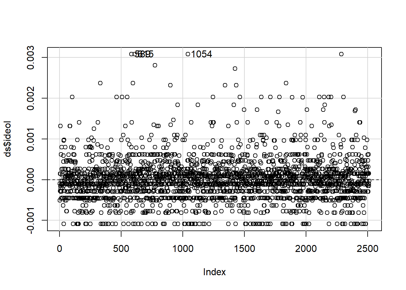
A useful method for finding dfbeta observations is to use the dfbetaPlots function in the car package. We specify the option id.n=2 to show the two largest df.betas. See figure 10.12.
plotdb<-dfbetaPlots(OLS_env, id.n=3)
#  Check the observations with high dfbetas.
#  We see the values 589 and 615 returned.
#  We only want to see results from columns gccrsk and ideology in tbur.data.
ds[c(589,615),c("glbcc_risk", "ideol")]
## glbcc_risk ideol
## 589 0 2
## 615 0 2These observations are interesting because they identify a potential problem in our model specification. Both observations are considered outliers because the respondents self-identified as “liberal” (ideology = 1) and rated their perceived risk of global climate change as 0. These values deviate substantially from the norm for other strong liberals in the dataset. Remember, as we saw earlier, our model has a problem with non-linearity – these outlying observations seem to corroborate this finding. The examination of outliers sheds some light on the issue.
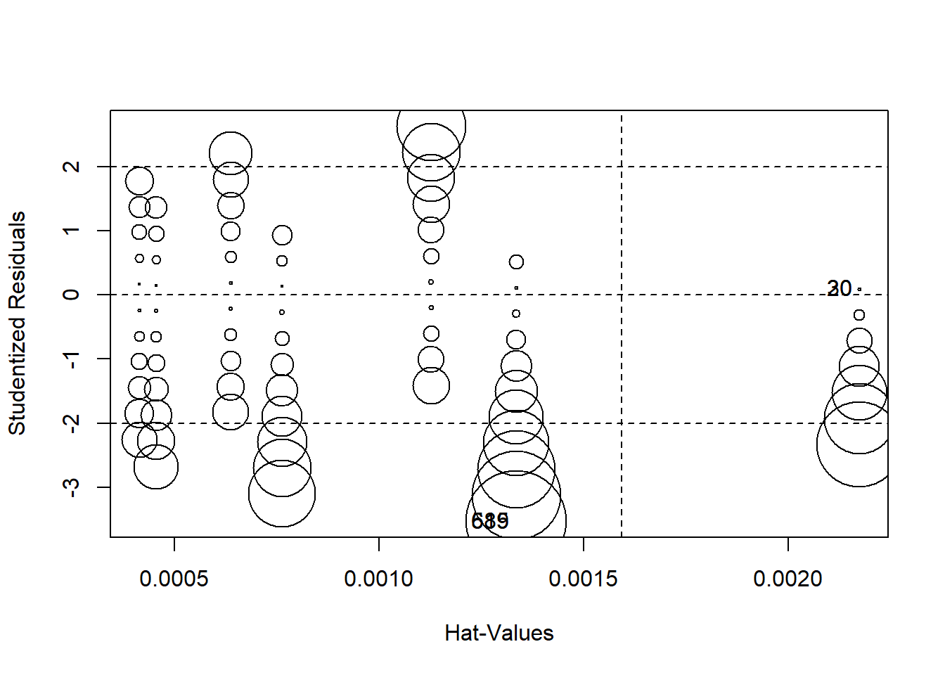
Finally, we can produce a plot that combines studentized residuals, “hat values”, and Cook’s D distances (these are measures of the amount of influence observations have on the model) using circles as an indicator of influence – the larger the circle, the greater the influence. Figure \(\PageIndex{13}\) displays the combined influence plot. In addition, the influencePlot the function returns the values of the greatest influence.
influencePlot(OLS_env)
##         StudRes         Hat          CookD
## 20   0.09192603 0.002172497 0.000009202846
## 30   0.09192603 0.002172497 0.000009202846
## 589 -3.53030574 0.001334528 0.008289418537
## 615 -3.53030574 0.001334528 0.008289418537
Figure \(\PageIndex{13}\) indicates that there are a number of cases that warrant further examination. We are already familiar with 589 and 615 Let’s add 20, 30, 90 and 1052.
#review the results
ds[c(589,615,20,30,90,1052),c("glbcc_risk", "ideol")]
## glbcc_risk ideol
## 589 0 2
## 615 0 2
## 20 10 1
## 30 10 1
## 90 10 1
## 1052 3 6One important take-away from a visual examination of these observations is that there do not appear to be any completely mis-coded or invalid data affecting our model. In general, even the most influential observations do not appear to be implausible cases. Observations 589 and 615 19 present an interesting problem regarding the theoretical and model specifications. These observations represent respondents who self-reported as “liberal” (ideology=2) and also rated the perceived risk of global climate change as 0 out of 10. These observations therefore deviate from the model’s expected values (“strong liberal” respondents, on average, believed global climate change represents a high risk). Earlier in our diagnostic testing, we found a problem with non-linearity. Taken together, it looks like the non-linearity in our model is due to observations at the ideological extremes. One way we can deal with this problem is to include a squared ideology variable (a polynomial) in the model, as illustrated earlier in this chapter. However, it is also important to note this non-linear relationship in the theoretical conceptualization of our model. Perhaps there is something special about people with extreme ideologies that need to be taken into account when attempting to predict the perceived risk of global climate change. This finding should also inform our examination of post-estimation predictions – something that will be covered later in this text.


